June 08, 2022
This article is part 3/13 (?) of a series of articles named Deep Learning with Python.
In this series, I will read through the second edition of Deep Learning with Python by François Chollet. Articles in this series will sequentially review key concepts, examples, and interesting facts from each chapter of the book.
Table of Contents
This chapter covers...
This chapter gives us everything required to get started with deep learning. By the end of this chapter, we'll be ready to move on to practical, real-world applications of deep learning.
TensorFlow is a free and open-source machine learning framework for Python. It was primarily developed by Google. Similar to NumPy, it is a general-purpose and efficient numerical library used by engineers to manipulate mathematical expressions using numerical tensors.
TensorFlow far surpasses NumPy in the following ways:
GradientTape)TensorFlow is much more than a single Python library. Rather, it's a platform home to a vast ecosystem of components, including:
Together, these components cover a wide range of use cases: from cutting-edge research to large-scale production, or just a simple image classification application to distinguish between a dog or a cat.
Scientists from Oak Ridge National Lab have used TensorFlow to train an extreme weather forecasting model on the 27,000 GPUs within the IBM Summit supercomputer. Google, on the other hand, has used TensorFlow to develop deep learning applications such as the chess-playing and Go-playing agent AlphaZero.
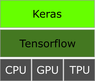
Keras is a high-level deep learning API built on top of TensorFlow. It provides a convenient and flexible API for building and training deep learning models.
Keras is known for providing a clean, simple, and efficient API that prioritizes the developer experience. It's an API for human beings, not machines, and follows best practices for reducing cognitive load. The API provides consistent and simple workflows, minimizes the number of actions required for common use cases, and outputs clear and actionable feedback upon user error.
Much like Python, Keras' large and diverse user base enables a well-documented and wide range of workflows for utilizing the API. Keras does not force one to follow a single "true" way of building and training models. Rather, it allows the user to build and train models corresponding to their preference, and to explore the possibilities of each approach.
Keras was designed originally in March 2015 to be used with Theano, a tensor-manipulation library developed by Montreal Institute for Learning Algorithms (MILA). Theano pioneered the idea of using static computation graphs for automatic differentiation and compiling code to both CPU and GPU support.
Following the release of TensorFlow 1.0 in November 2015, Keras was refactored to support multiple backend architectures: starting with Theano and TensorFlow in late 2015, and adding support for CNTK and MXNet in 2017.
Keras became well known as the user-friendly way to develop TensorFlow applications. By late 2017, a majority of TensorFlow users were using Keras. In 2018, the TensorFlow leadership picked Keras as TensorFlow's official high-level API. As of September 2019, the Keras API is the official API for TensorFlow 2.0.
Enough of the history, let's learn how to set up a deep learning workspace.
There are a handful of ways to set up a deep learning workspace:
Each approach has its advantages and disadvantages in terms of flexibility, cost, and ease of use. I'll briefly discuss the advantages and disadvantages of each approach below, but I will not discuss setup at all. In short, the easiest way to get started is Google Colab or some cloud GPU instance.
Buying a machine with a GPU is not the easiest way to get started with DL, as it's the most expensive upfront and requires manual setup. The upfront cost is amplified by the current (as of June 2022) chip shortage and GPU scalpers. This method involves installing proper drivers, sorting out version conflicts, and then configuring the libraries to use the GPU instead of the CPU.
Most users already have NVIDIA GPUs installed on their computers. Given the large user base of TensorFlow, there are many tutorials for setting up NVIDIA GPUs for deep learning, so this is not a bad option for tech-savvy people. I run most of my deep learning code on my GPU as it's the most convenient option and does not require an internet connection.
The alternative to buying a GPU is the use of embedded devices built specifically for efficient and highly-parallelized math operations, such as NVIDIA's Jetson or Google's Coral.
Using GPU instances is cheaper in the short term because you pay as you go (per hour basis), but it's not sustainable in the long run if you're a heavy user of deep learning. The benefit of using GPU instances is that it requires minimal setup as most instances have Python, TensorFlow, and Keras pre-installed - it's mostly plug-and-play and easy to use. Moreover, the GPU instance can easily be upgraded, torn down, cloned, and re-installed. Lastly, students and enterprise employees often get discounts - or free usage - for AWS and Google Cloud.
I use Jarvis Labs and AWS for my deep learning needs because I have discounts for both services. There aren't many differences between cloud instance providers other than the availability of high-powered GPUs.
The last approach - using free GPUs from Google Colab - is the simplest way to get started with deep learning. It's recommended for those who are not familiar with the hardware and software, and for those who are new to deep learning. Francois himself recommends executing code examples found in the book using Google Colab as it requires the least amount of setup. The drawback of Colab is that the free GPU is time-limited and shared by users - meaning that the execution may be slower.
Training a neural network revolves around low-level tensor manipulations and high-level deep learning concepts. TensorFlow takes care of the tensor manipulation through the use of:
relu, matmul, etc.
GradientTape)
Let's take a deeper dive into how all of the concepts above translate to TensorFlow.
To do anything in TensorFlow, we need to create tensors. Let's look at code examples for creating tensors with all ones, zeros, or random values:
import tensorflow as tf

# Equivalent to np.ones((2, 2))
t_ones = tf.ones(shape=(2, 2))
# Equivalent to np.zeros((2, 1))
t_zeros = tf.zeros(shape=(2, 1))
# Equivalent to np.random.normal(size=(3, 1), loc=0., scale=1)
t_random_normal = tf.random.normal(shape=(3, 1), mean=0., stddev=1.)
# Equivalent to np.random.uniform(size=(1, 3), low=0., high=1.)
t_random_uniform = tf.random.uniform(shape=(1, 3), minval=0., maxvval=1.)
What do the outputs of each tensor look like?
>>> print(t_ones)
tf.Tensor(
    [[1. 1.]
     [1. 1.]], shape=(2, 2), dtype=float32)

>>> print(zeros)
tf.Tensor(
    [[0.]
     [0.]], shape=(2, 1), dtype=float32)

>>> print(t_random_normal)
tf.Tensor(
    [[-0.8276905]
     [ 0.2264915]
     [ 0.1399505]], shape=(3, 1), dtype=float32)

>>> print(t_random_uniform)
tf.Tensor(
    [[0.141 0.824 0.912]], shape=(1, 3), dtype=float32)
A significant difference between NumPy arrays and TensorFlow tensors is that tensors are not assignable: they're
constant.
For instance, in NumPy, we can assign a value to a tensor, as seen in the code block below.
Whereas, in TensorFlow, we are greeted with an error:
TypeError: 'Tensor' object does not support item assignment.
>>> import numpy as np
>>> t_ones = np.ones((2, 2))
>>> t_ones
array([[1., 1.],
       [1., 1.]])
>>> t_ones[0, 0] = 0
>>> t_ones
array([[0., 1.],
       [1., 1.]])

>>> import tensorflow as tf
>>> t_ones = tf.ones((2, 2))
>>> t_ones
tf.Tensor(
    [[1. 1.]
     [1. 1.]], shape=(2, 2), dtype=float32)
>>> t_ones[0, 0] = 0
Traceback (most recent call last):
  File "<stdin>", line 1, in <module>
TypeError: 'Tensor' object does not support item assignment
To train a model, however, it's important to be able to change the values of the tensors - update the weights of
the model.
This is where the TensorFlow's variable (tf.Variable) comes into play:
>>> v = tf.Variable(initial_value=tf.random.normal(shape=(3, 1)))
>>> print(v)
array([[-0.644994 ],
       [ 1.47064  ],
       [-0.6413262]], dtype=float32)>
The state of a variable - the entirety of or a subset of coefficients - can be modified via its
assign method:
>>> v.assign(tf.ones((3, 1)))
array([[1.],
       [1.],
       [1.]], dtype=float32)>
>>> v[0,0].assign(9)
array([[9.],
       [1.],
       [1.]], dtype=float32)>
Similarly, the assign_add() and assign_sub() are tensor-efficient equivalents of
+= and -=, respectively.
>>> v.assign_add(tf.ones((3, 1)))
array([[10.],
       [ 2.],
       [ 2.]], dtype=float32)>
>>> v.assign_sub(tf.ones((3, 1)))
array([[9.],
       [1.],
       [1.]], dtype=float32)>
TensorFlow's ability to retrieve gradients of any expression with respect to any of its inputs is what makes the
TensorFlow library so powerful.
All we have to do is open a GradientTape context, manipulate the input tensors, and retrieve the
gradients with respect to the inputs.
import tensorflow as tf

input_var = tf.Variable(initial_value=3.)
# Open a GradientTape context
with tf.GradientTape() as tape:
    # Manipulate the input tensor
    output = input_var * input_var

# gradient = <tf.Tensor: shape=(), dtype=float32, numpy=6.0>
gradient = tape.gradient(output, input_var)
The gradient tape is most commonly used to retrieve the gradients of the model's loss with respect to its
weights: gradient = tape.gradient(loss, weights).
We discussed and demonstrated this functionality in the previous
article.
So far, we've only looked at the simplest case of GradientTapes - where the input tensors in
tape.gradient() were TensorFlow variables.
It's possible for the input tensors to be any arbitrary tensor, not just variables, by calling
tape.watch(arbitrary_tensor) within the GradientTape context.
arbitrary_tensor = tf.constant(value=2.)
with tf.GradientTape() as tape:
    tape.watch(arbitrary_tensor)
    output = arbitrary_tensor * arbitrary_tensor

# tf.Tensor(4.0, shape=(), dtype=float32)
gradient = tape.gradient(output, arbitrary_tensor)
By default, only trainable variables are tracked because it would be too expensive to preemptively store the information required to compute the gradient of anything with respect to anything. To avoid wasting resources, only the trainable variables are tracked unless otherwise explicitly specified.
The gradient tape is a powerful utility capable of computing second-order gradients - or, the gradient of a gradient.
For instance, the gradient of an object's position with respect to time is the object's speed. The second-order gradient of the object's speed is its acceleration.
time = tf.Variable(initial_value=0.)
with tf.GradientTape() as outer_tape:
    with tf.GradientTape() as inner_tape:
        position = 4.9 * time ** 2
    speed = inner_tape.gradient(position, time)

# <tf.Tensor: shape=(), dtype=float32, numpy=9.8>
acceleration = outer_tape.gradient(speed, time)
We now know about tensors, variables, tensor operations, and gradient computation. That's enough to build any machine learning model based on gradient descent. Let's put our knowledge to the test and build an end-to-end linear classification model purely in TensorFlow.
We're going to implement a linear classifier that predicts whether a given input belongs to class A or class B. But first, we need to understand what linear classification is.
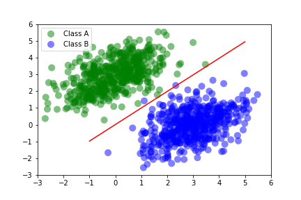
In linear classification problems, the model is trying to find a linear combination of the input features that best predicts the target variable. Simply put, the model is trying to classify input data into 2+ categories (classes) by drawing a line through the data. The line best fits to separate the data into two classes.
We see in the figure to the right how the model classifies the two classes with a red line. Inputs above the red line belong to class A and inputs below the line belong to class B. There are a few class B outliers above the line, but remember that the classification line is best fit, not perfect fit.
This is the basic idea behind linear classification. Now let's generate some data and train a linear classifier. All of the code related to this linear classifier can be found on my GitHub as an interactive python file. I recommend using VSCode to utilize the interactive python code blocks - similar to Jupyter Notebooks.
We need some nicely linear data to train our linear classifier. To keep it simple, we'll create two classes of points in a 2D plane and call them class A and class B. To keep it more simple, we won't explain all the math behind the data generation - just understand that both classes should be clearly separated and roughly distributed like a cloud. We'll use the following formula to generate the data:
num_samples_per_class = 500
class_a_samples = np.random.multivariate_normal(
    mean=[0, 3],
    cov=[[1, 0], [0, 1]],
    size=num_samples_per_class)
class_b_samples = np.random.multivariate_normal(
    mean=[3, 0],
    cov=[[1, 0], [0, 1]],
    size=num_samples_per_class)
The figure below shows the linearly-separable data of classes A and B. See the following code block to see how we plot the data.
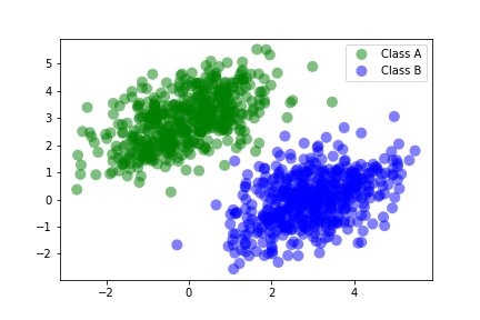
Both samples are matrices of shape (500, 2) - meaning there are 500 rows of 2-dimensional data (aka
500 vectors/tuples, each containing an x,y).
Let's stack both class samples into a single array with the shape (1000, 2).
Stacking the samples into a single array will allow for easier processing later on, such as plotting the data.
import matplotlib.pyplot as plt
import numpy as np

# The first 500 samples are from class A, the next 500 samples are from class B
inputs = np.vstack((class_a_samples, class_b_samples)).astype(np.float32)
# The first 500 labels are 0 (class A), and the next 500 are 1 (class B)
labels = np.vstack(
    (
        np.zeros((num_samples_per_class, 1), dtype=np.float32),
        np.ones((num_samples_per_class, 1), dtype=np.float32),
    )
)
class_a = inputs[:num_samples_per_class]
class_b = inputs[num_samples_per_class:]

# %% Plot the two classes
# Class A is represented by green dots, and class B is represented by blue dots,
# plt.scatter(inputs[:, 0], inputs[:, 1], c=labels[:, 0], s=100)
plt.scatter(
    class_a[:, 0],
    class_a[:, 1],
    c="green",
    alpha=0.50,
    s=100,
    label="Class A",
    edgecolors="none",
)
plt.scatter(
    class_b[:, 0],
    class_b[:, 1],
    c="blue",
    alpha=0.50,
    s=100,
    label="Class B",
    edgecolors="none",
)
plt.legend()
plt.savefig("../img/linear_classifier_data.png", transparent=False)
plt.show()
A linear classifier is an affine transformation of the input data
(prediction = dot(W, x) + b), trained to minimize the square of the difference (mean squared error,
or MSE) between the prediction and the target label.
I have not explained affine transformations - or any geometric interpretations of tensor operations - in my articles, but François Chollet greatly details geometric transformations in Chapter 2 of his book. In short, an affine transformation is the combination of a linear transform (dot product) and a translation (vector addition).
Now that we understand the basic math behind linear classification, let's create the model's variables, forward pass, and loss function.
input_dim = 2   # input is a 2D vector
output_dim = 1  # output is a scalar, class B < 0.5 < class A
W = tf.Variable(initial_value=tf.random.uniform(shape=(input_dim, output_dim)))
b = tf.Variable(initial_value=tf.zeros(shape=(output_dim,)))
Our forward pass function is the affine transformation discussed above. Our loss function is the mean squared error (MSE) between the prediction and the target label.
def model(inputs) -> tf.Tensor:
    return tf.matmul(inputs, W) + b

def square_loss(predictions, targets) -> tf.Tensor:
    # Calculate the loss per sample, results in tensor of shape (len(targets), 1)
    per_sample_loss = tf.square(targets - predictions)
    # Average the per-sample loss and return a single scalar loss value
    return tf.reduce_mean(per_sample_loss)
Next, we have to train the model.
Let's create the training step, where the model's weights and biases are updated based on the loss.
def training_step(inputs, targets, learning_rate: float = 0.001) -> tf.Tensor:
    with tf.GradientTape() as tape:
        predictions = model(inputs)
        loss = square_loss(predictions, targets)
    # Calculate the gradients of the loss with respect to the variables
    grad_loss_wrt_W, grad_loss_wrt_b = tape.gradient(loss, [W, b])
    # Update the variables using the gradients and the learning rate
    W.assign_sub(learning_rate * grad_loss_wrt_W)
    b.assign_sub(learning_rate * grad_loss_wrt_b)
    return loss
Finally, let's create the training loop. For simplicity, we'll do batch training instead of mini-batch training. Batch training means the model trains on all the data at once instead of iteratively over small batches of the data.
Batch training has its pros and cons: each training step will take much longer to run since we'll compute the forward pass and gradient calculation for the entire dataset (1000 samples in our example). On the other hand, because the model is training on the entire dataset, each gradient update will be much more effective at reducing the loss since it learns information from all training samples.
num_epochs = 50
# Save the loss scores so we can plot them later
loss_all = []
# Save all predictions so we can calculate and plot the accuracy later
predictions_all = []

for step in range(num_epochs):
    step_loss = training_step(inputs=inputs, targets=labels)
    print(f"Step {step} loss: {step_loss}")
    loss_all.append(step_loss)
    predictions_all.append(model(inputs))
Full output of loss scores
Step 0: Loss = 2.9617
Step 1: Loss = 0.4816
Step 2: Loss = 0.1756
Step 3: Loss = 0.1239
Step 4: Loss = 0.1098
Step 5: Loss = 0.1017
Step 6: Loss = 0.0950
Step 7: Loss = 0.0890
Step 8: Loss = 0.0836
Step 9: Loss = 0.0785
Step 10: Loss = 0.0740
Step 11: Loss = 0.0698
Step 12: Loss = 0.0660
Step 13: Loss = 0.0625
Step 14: Loss = 0.0593
Step 15: Loss = 0.0563
Step 16: Loss = 0.0536
Step 17: Loss = 0.0512
Step 18: Loss = 0.0490
Step 19: Loss = 0.0469
Step 20: Loss = 0.0450
Step 21: Loss = 0.0433
Step 22: Loss = 0.0418
Step 23: Loss = 0.0403
Step 24: Loss = 0.0390
Step 25: Loss = 0.0378
Step 26: Loss = 0.0367
Step 27: Loss = 0.0357
Step 28: Loss = 0.0348
Step 29: Loss = 0.0340
Step 30: Loss = 0.0332
Step 31: Loss = 0.0325
Step 32: Loss = 0.0319
Step 33: Loss = 0.0313
Step 34: Loss = 0.0307
Step 35: Loss = 0.0302
Step 36: Loss = 0.0298
Step 37: Loss = 0.0294
Step 38: Loss = 0.0290
Step 39: Loss = 0.0287
Step 40: Loss = 0.0284
Step 41: Loss = 0.0281
Step 42: Loss = 0.0278
Step 43: Loss = 0.0272
Step 44: Loss = 0.0268
Step 45: Loss = 0.0261
Step 46: Loss = 0.0259
Step 47: Loss = 0.0255
Step 48: Loss = 0.0254
Step 49: Loss = 0.0254
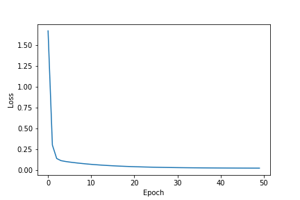
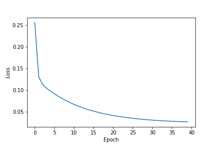
After 50 epochs, or 50 training steps, the loss score stabilizes to around 0.025. Let's plot the loss scores to see how the loss score changes after each training step.
It's difficult to see the rate of decrease in the loss score following the rapid convergence after step 0 and long tail. The initial loss score was initially at 2.9617 on step 0 and dropped to 0.4816 on step 1. We can improve the plot by excluding the initial loss score and "trimming" the long tail at the point where see the score stabilizes (~40 epochs). Let's clean up the data and plot the loss scores so we can better visualize the rate of decrease.
plt.plot(loss_all[1:41])
plot.xlabel("Epoch")
plot.ylabel("Loss")
|
|
| Loss scores of all training steps, converges to ~0.025 after roughly 40 epochs | All loss scores, excluding the initial loss score and trimming the plot's long tail |
Can we train the model for more epochs and make it more accurate?
No. Take a look at the plots above: the loss score stabilizes after roughly 40 epochs.
The stabilization shows that the model learned its optimal weights given the current model architecture and training data. If we were to train it for more epochs, the model would overfit (memorize) to the data.
Overfitting is a huge concept in machine learning, which we'll cover later on. For now, understand that more training does not guarantee better results! Training with a quality dataset and decently-configured model architecture is more impactful than excessive training.
After each training step - each iteration over the entire dataset - the model updates its weights and biases
(parameters) and makes predictions on the inputs.
We append those predictions to a list called predictions_all.
Using the predictions, we can plot model's accuracy after each training step: green dot if correctly predicted,
red otherwise.
Predictions are classified as correct or incorrect based on the following criteria:
An easier way to understand this is: if the dot is above the red line, it belongs to class A, otherwise it's below the line and belongs to class B.
We need two helper functions to create the accuracy plots and GIFs below:
plot_prediction_acc(prediction, input) and make_gif(predictions, inputs).
The plot_prediction_acc() function will plot the accuracy of the model and save it to an IO buffer.
The make_gif() function will create a GIF from the IO buffer and save it to a file.
Easy peasy.
import matplotlib.pyplot as plt
import numpy as np

# %% Scatter plot for the model's predictions where the dots are green if the prediction is accurate, red if the prediction is incorrect
def plot_prediction_acc(
    prediction: np.ndarray,
    inputs: np.ndarray,
    buffer=None,
    parameters: tuple[np.ndarray, float] = None,
    savename: str = "",
    title: str = "",
):
    plt.scatter(
        inputs[:, 0],
        inputs[:, 1],
        c=[
            "green" if labels[idx] == pred else "red"
            for idx, pred in enumerate(prediction > 0.5)
        ],
        alpha=0.20,
        s=100,
    )
    # Draw the red line separating the two classes
    if parameters:
        W, b = parameters
        x = np.linspace(-1, 5, 100)
        y = -W[0] / W[1] * x + (0.5 - b) / W[1]
        plt.plot(x, y, c="red")
        plt.xlim(-3, 6)
        plt.ylim(-3, 6)
    # Add a title to the plot
    if title:
        plt.title(title)
    # Save the plot to a file
    if savename:
        plt.savefig(f"../img/{savename}.png", transparent=False)
    # Save the plot to a buffer
    if buffer:
        plt.savefig(buffer, format="png", transparent=False)
    else:
        plt.show()
    plt.close()


# %% Make gif
make_gif(predictions_all, inputs, "prediction_accuracy")
How to make a GIF of matplotlib plots
There are many ways to make a GIF of matplotlib plots.
Matplotlib even has an animation module (here) that can be used to make GIFs.
However, it's not intuitive enough for me to use at the moment, so I hacked together something I knew would
work using imageio and io.BytesIO.
Please refer to the code block below to view my implementations of make_gif.
There are two different implementations:
make_gif appends each image to the writer object (imageio.get_writer())make_gif_with_duration appends each image to a list and passes the list to
imageio.mimsave()
A third implementation to better generalize and enhance this function: save all the prediction images outside
of the function and pass the list of images to make_gif instead of the list of predictions.
Therefore, we'd only have to make each image one time and save computational resources.
from io import BytesIO
import imageio


def make_gif(predictions: np.ndarray, inputs: np.ndarray, savename: str):
    fig, ax = plt.subplots()

    with imageio.get_writer(f"../img/{savename}.gif", mode="I") as writer:
        # for prediction_idx in [0, 1, 2, -1]:
        for prediction_idx, prediction in enumerate(predictions):
            params = parameters_all[prediction_idx]
            buffer = BytesIO()
            plot_prediction_acc(
                prediction=prediction,
                inputs=inputs,
                buffer=buffer,
                parameters=params,
                title=f"Prediction {prediction_idx}",
            )
            buffer.seek(0)
            img = plt.imread(buffer, format="png")
            writer.append_data(img)

    plt.show()

# Slow down the GIF by increasing the `duration` argument to 0.5 or 1 (seconds)
def make_gif_with_duration(
    predictions: np.ndarray, inputs: np.ndarray, savename: str, duration: float
):
    images = []
    for prediction_idx, prediction in enumerate(predictions):
        params = parameters_all[prediction_idx]
        buffer = BytesIO()
        plot_prediction_acc(
            prediction=prediction,
            inputs=inputs,
            buffer=buffer,
            parameters=params,
            title=f"Prediction {prediction_idx}",
        )
        buffer.seek(0)
        images.append(plt.imread(buffer, format="png"))
    imageio.mimsave(f"../img/{savename}.gif", images, duration=duration)
In the following plots, we see green dots representing correct predictions and red dots representing incorrect predictions. After each training step, the model adjusts its parameters causing the red class-separation line to gradually adjust in the direction of the correct prediction. As training continues, the number of incorrect predictions decreases, and the line properly separates the two classes. Pretty cool, right?
|

|
| Accuracy of the first 20 predictions, slowed down | Accuracy of all predictions |
This is what linear classification is all about: finding the parameters of a line that neatly separates two classes of data. In higher-dimensional spaces, we're finding the parameters of a hyperplane that neatly separates the two classes.
We've learned how to create a linear classifier using pure TensorFlow. Now, let's look closer at Keras - specifically, the anatomy of a neural network through Keras layers and models.
A layer is the fundamental data structure in neural networks. As discussed in chapter 2, a layer is a data processing module that takes as input one or more tensors and outputs one or more tensors. We previously referred to layers as a "data filter" where data goes in and comes out more useful. Everything in Keras is either a layer or something that closely interacts with a layer.
Some layers can be stateless, but layers are more commonly stateful. The layer's state may contain weights which represent the network's knowledge.
Furthermore, different types of layers are appropriate for different tensor formats and data processing tasks:
Dense, or fully-connected, layers often process vector data stored in 2D tensors of shape
(samples, features)
LSTM (long short-term memory) or Conv1D (1D convolution
layer), often process time-series data stored in 3D tensors of shape
(samples, timesteps, features)
Conv2D (2D convolution layer) and Conv3D (3D convolution layer) often process
images stored in 4D tensors of shape (samples, height, width, channels)Tensor formats were discussed in more detail in the previous article.
In Keras, a Layer is an object that encapsulates some state (weights) and some computation (a
forward pass).
The weights are typically defined in a build() method - although they could be created in the
constructor.
The computation, or forward pass, is defined in the call() method.
from tensorflow import keras


class SimpleDense(keras.layers.Layer):
    def __init__(self, units, activation=None, **kwargs):
        super().__init__(**kwargs)
        self.units = units
        self.activation = keras.activations.get(activation)

    def build(self, input_shape):
        input_dim = input_shape[-1]
        # self.kernel = tf.Variable(tf.random.normal(shape=(input_dim, self.units)))
        self.kernel = self.add_weight(
            shape=(input_dim, self.units),
            initializer="random_normal",
            name="weights"
        )
        self.bias = self.add_weight(
            shape=(self.units,),
            initializer="zeros",
            name="bias"
        )

    def call(self, inputs):
        # return self.activation(keras.backend.dot(inputs, self.kernel) + self.bias)
        y = tf.matmul(inputs, self.kernel) + self.bias
        if self.activation is not None:
            y = self.activation(y)
        return y

my_dense = SimpleDense(units=32, activation="relu")
input_tensor = tf.ones(shape=(2, 32))
output_tensor = my_dense(input_tensor)
output_tensor.shape
Once instantiated, a layer can be called on a tensor to produce a new tensor.
>>> my_dense = SimpleDense(units=32, activation="relu")
>>> input_tensor = tf.ones(shape=(2, 784))
>>> output_tensor = my_dense(input_tensor)
>>> output_tensor.shape
TensorShape([2, 32])
>>> output_tensor.numpy()
array([[0.        , 0.16681111, 0.37626198, 0.32816353, 0.        ,
        ...
        0.        , 0.16670324],
       [0.        , 0.16681111, 0.37626198, 0.32816353, 0.        ,
        ...
        0.        , 0.16670324]], dtype=float32)
When do we call the build() method? How are the weights created?
We don't have to explicitly call the build() method because it's handled by the superclass.
The weights are built - and build() called automatically - the first time the layer is called.
The superclass's __call__() method calls the build() method if the layer has not been
built yet.
def __call__(self, inputs):
    if not self.built:
        self.build(inputs.shape)
        self.built = True
    return self.call(inputs)
That's the gist of Keras layers. Let's talk about model architectures.
Simply put, a deep learning model, such as the Model class in Keras, is a graph of layers.
Until now, we've only discussed Sequential models - a linear stack of layers that map a single
input to a single output.
As we move forward, we'll be exposed to a variety of neural network architectures:
The difference between each of these topologies is the type of layers and how they are connected. Each network topology has its pros, cons, and common use cases. Picking the right network topology is more an art than a science, where only practice can help you become a proper neural network architect.
Why is it important to pick a proper network architecture for my use case?
To learn from data, we have to make assumptions about it - also referred to as a hypothesis space or space of possibilities in chapter 1. These assumptions (hypothesis space) define what can be learned. By choosing a network topology, we constrain our hypothesis space to a specific series of tensor operations. As such, the architecture of the model is extremely important for constraining what our model can learn - how it can make proper assumptions.
The hypothesis space encodes the assumptions we make about our problems, aka the prior knowledge that the model
starts with.
For instance, if we're working on a two-class classification problem with a model made of a single
Dense layer with no activation function, then we are assuming that our two classes are linearly
separable.
Finding the right balance between the number of layers, types of layers, and the number of parameters in the
model is a key part of choosing a network architecture.
In short, the network's architecture constrains the data that can be learned. We must find the right architecture for our problem and data. With time, this process will become second nature.
Enough of model architecture, let's talk about model compilation and how we configure the learning process.
Once the model architecture is defined, there are three more key parts to be defined:
Once we've defined the loss function, optimizer, and metrics, we can begin training the model using the
model.compile() and model.fit() methods.
Alternatively, we could write our custom training loops instead of using the model.fit() method,
but that's covered in chapter 7.
For now, let's take a look at the compile() method.
The compile() method configures the training process using the arguments optimizer,
loss, and metrics (a list):
model = keras.Sequential([keras.layers.Dense(1)])
model.compile(optimizer="rmsprop", loss="mean_squared_error", metrics=["accuracy"])
One important thing to note is how we pass in the arguments to the compile() method.
In the example above, we passed them in as strings and the method is flexible enough to understand what we want.
However, rather than passing in a string, we can also pass in objects.
model.compile(
    optimizer=keras.optimizers.RMSprop(learning_rate=0.001),
    loss=keras.losses.MeanSquaredError(),
    metrics=[keras.metrics.BinaryAccuracy()]
)
Passing in objects is useful when we want to use a custom object, such as a custom loss function or optimizer. As stated above, customizing the training process will be discussed in chapter 7. In the meantime, please refer to the Keras documentation regarding built-in options for optimizers, loss functions, and metrics.
Choosing the proper loss function for the right problem is a critical step in training a model. Neural networks will take any shortcut they can to minimize the loss score, even if it means learning the wrong thing and performing incorrectly. The network will end up doing things we did not intend it to do. Read more about how "smart" neural networks can be in OpenAI's article about specification gaming.
Common problems - such as classification, regression, and timeseries prediction (forecasting) - all have general guidelines for choosing a loss function. For instance, the mean squared error is a good choice for regression problems. The binary cross-entropy is a good choice for two-class classification problems, whereas the categorical cross-entropy is a good choice for multi-class classification problems. Only when we have a problem that is not one of these common problems will we need to develop a custom loss function.
In the next few chapters, we'll detail explicitly which loss functions to choose for a wide range of common problems.
After compiling the model, we can fit it to data by calling the fit() method.
The fit() method implements the training loop using a few key arguments:
data (inputs and targets) to train on. Data is typically passed in as a Numpy array or
TensorFlow Dataset object.epochs to train for: how many times the training loop should iterate over the
entire dataset.history = model.fit(
inputs, targets, epochs=10, batch_size=32
)
train_dataset = image_dataset_from_directory(
TRAIN_DIR,
image_size=(600, 200),
# batch_size=16
)
validation_dataset = image_dataset_from_directory(
VALIDATE_DIR,
image_size=(600, 200),
# batch_size=16
)
history = model.fit(
train_dataset,
epochs=50,
validation_data=validation_dataset,
)
NOTE: TensorFlow Dataset object
The Dataset object will be covered in depth in later chapters. However, it's important to understand that the Dataset object is a wrapper around a Python generator. The Dataset is powerful and simple at the same time. Read more about the Dataset object in the TensorFlow guide or TensorFlow API documentation.
The fit() method returns a History object, which contains information about the
training process.
This object contains a dictionary (History.history) which maps training metrics, such as the loss
and accuracy, to their per-epoch values.
>>> history.history
{'loss': [0.988, 0.878, 0.632, 0.498, ...],
 'accuracy': [0.001, 0.283, 0.401, 0.651, ...]}
This dictionary is used to plot the training loss and accuracy during training.
The goal of machine learning is to obtain models that perform well on both training data and unseen data. Just because the model performs well on the training data, it does not mean it can perform well on new, unseen data.
To understand how the model performs on unseen data, it's standard practice to reserve a subset of the training data as validation data. The validation data is used for computing the loss value and metrics, whereas the training data is used for updating the model's weights (training the model).
We can utilize the fit() method's validation_data argument to monitor the model's
performance on our validation data.
Similar to the training data, the validation data can be passed in as a Numpy array or a TensorFlow Dataset
object.
# Reserve 25% of training data for validation
num_validation_samples = len(0.25 * len(inputs))

# Create training and validation datasets
training_targets = targets[:num_validation_samples]
training_inputs = inputs[:num_validation_samples]
validation_inputs = inputs[num_validation_samples:]
validation_targets = targets[num_validation_samples:]
validation_data = (validation_inputs, validation_targets)

# Train the model
history = model.fit(
    training_inputs, training_targets,
    epochs=10,
    batch_size=32,
    validation_data=validation_data  # Can be a tuple (inputs, targets) or a Dataset object
)
During training, the model will be trained on the training data and then evaluated on the validation data.
As a result, the history.history object will contain the loss and accuracy values for both the
training and validation data.
NOTE: Keep training and validation data strictly separated
The purpose of validation is to monitor whether what the model is learning is useful for new data. If any of the validation data has already been seen by the model during training, the model's validation loss and accuracy will be flawed.
If instead, we wanted to compute the model's validation loss and metrics after the training loop has
finished, we can use the evaluate() method.
evaluate() iterates over the data passed in batches and returns a list of scalars, where the first
scalar is the loss and the second is the accuracy.
# Evaluate the model on validation data
loss_and_metrics = model.evaluate(validation_inputs, validation_targets, batch_size=32)
loss = loss_and_metrics[0]
metric = loss_and_metrics[1]
Now that the model is trained, it can be used to make predictions on new data.
The model can now be used to make predictions on new data in two ways:
__call__() method:
model(inputs)
predict(inputs, batch_size) method, which returns a Numpy array of predictions:
model.predict(inputs, batch_size)
>>> predictions = model(inputs)
>>> predictions = model.predict(inputs, batch_size=64)
>>> print(predictions[:3])  # Print first 3 predictions
[[0.124155,
  0.298401
  0.695342,]]
Training a model isn't as difficult as it sounds. This is all we need to know about the Keras API for now. We're now ready to start building models for real-world problems.
The following chapter will discuss how to build neural networks for classification and regression problems.
Layer class.
A layer encapsulates some weights and some computation.
Models are composed of layers.model.compile() methodmodel.fit() method.
It's common practice to train the model on the training data and to monitor the model's performance on the
validation data - a set of inputs that have not been seen by the model.model.predict(inputs, batch_size) to make predictions on new data.