Sample image

May 9, 2022
This article is part 2/13 (?) of a series of articles named Deep Learning with Python.
In this series, I will read through the second edition of Deep Learning with Python by François Chollet. Articles in this series will sequentially review key concepts, examples, and interesting facts from each chapter of the book.
Table of Contents
This chapter covers...
Understanding deep learning requires familiarity with many simple mathematical concepts: tensors, tensor operations, differentiation, gradient descent, and so on. This chapter will build on the concepts above without getting overly technical. The use of precise, unambiguous executable code, instead of mathematical notation, will allow most programmers to easily grasp these concepts.
Concrete example of a neural network (NN) with the use of the Python library Keras to learn how to
classify handwritten digits.
The problem we're trying to solve here is to classify grayscale images of handwritten digits (28x28 pixels) into their 10 categories (digits 0 through 9). This problem is commonly referred to as the "Hello World" of deep learning - it's what you do to verify your algorithms are working as expected.
NOTE: Classification problem keywords
In ML classification problems, a category is called a class. Data points - such as individual train or test images - are called samples. The class associated with a specific sample is called a label.
We'll be using the MNIST dataset: a set of 60,000 training images, plus 10,000 test images, assembled by the National Institute of Standards and Technology (the NIST in MNIST) in the 1980s.
The MNIST dataset is preloaded in Keras, in the form of four NumPy arrays:
from tensorflow.keras.datasets import mnist
(train_images, train_labels), (test_images, test_labels) = mnist.load_data()
Let's take a peek at the shape of the data. We should see 60,000 training images and labels, 10,000 test images and labels.
>>> train_images.shape
(60000, 28, 28)
>>> len(train_labels)
60000
>>> train_labels
array([5, 0, 4, ..., 5, 6, 8], dtype=uint8)
>>>
>>> test_images.shape
(10000, 28, 28)
>>> len(test_labels)
10000
>>> test_labels
array([7, 2, 1, ..., 4, 5, 6], dtype=uint8)
Let's look at a sample image using the matplotlib library:
import matplotlib.pyplot as plt
digit = train_images[4]
plt.imgshow(digit, cmap=plt.cm.binary)
plt.show()
Sample image
Lastly, let's look at what label corresponds to the previous image:
>>> train_labels[4]
9
The core building block of a neural network is the layer. A layer can be considered as a data filter: data goes in and comes out more purified - more useful. Specifically, layers extract representations out of the input data.
In deep learning models, simple layers are chained together to form a data distillation network. Deep learning models could be visualized as a sieve for data processing - successive layers refining input data more and more.
The following example is a two-layer neural network. We aren't expected to know exactly what the example means - we'll learn throughout the next two chapters.
The model consists of a sequence of two Dense layers, which are densely connected (also called
fully connected).
The second layer is a 10-way softmax classification layer, which means it will return an array of 10
probability scores (summing to 1).
Each score will be the probability that the current digit image belongs to on our of 10 digit classes.
from tensorflow import keras
from tensorflow.keras import layers
model = keras.Sequential([
    layers.Dense(512, activation="relu"),
    layers.Dense(10, activation="softmax")
])
Before we begin training, we must compile three more things, in addition to the training and testing data, as part of the compilation step: We brushed over the jobs of the loss score and optimizer in the previous chapter. The specifics of their jobs will be made clear throughout the next two chapters.
model.compile(optimizer="rmsprop",
              loss="sparse_categorical_crossentropy",
              metrics=["accuracy"])
Before training, we'll preprocess the data to ensure consistent data shapes and scales during training. We'll reshape the data into the shape the model expects and scale it so that all values are in the [0, 1] interval instead of [0, 255] interval.
The training image data will transform from a uint8 array of shape (60000, 28, 28) with
values between [0, 255] to a float32 array of shape (60000, 28*28) with values between
[0, 1].
The same reshaping and reformatting process is applied to the testing image data.
train_images = train_images.reshape((60000, 28*28))
train_images = train_images.astype("float32") / 255
test_images = test_images.reshape((10000, 28*28))
test_images = test_images.astype("float32") / 255
With the data properly pre-processed, we are finally ready to train the model!
In Keras, training the model is done via a call to the model's fit() method - we fit the
model to its training data.
>>> model.fit(train_images, train_labels, epochs=5, batch_size=128)
Epoch 1/5
60000/60000 [==========================] - 5s - loss: 0.2524 - acc: 0.9273
Epoch 2/5
51328/60000 [====================>.....] - ETA: 1s - loss: 0.1035 - acc: 0.9692
The model swiftly reaches a decent accuracy of 96% after roughly 2 epochs of fitting to the training data.
Now that the model is trained, we can use it to make class predictions on the new, unseen data - such as the testing images.
>>> test_digit = test_images[0]
>>> prediction = model.predict(test_digit)
>>> prediction
array([1.0726176e-10, 1.6918376e-10, 6.1314843e-08, 8.4106023e-06,
       2.9967067e-11, 3.0331331e-09, 8.3651971e-14, 9.9999106e-01,
       2.6657624e-08, 3.8127661e-07], dtype=float32)
Each index i in predictions[0] corresponds to the probability that prediction
belongs to class i.
In this example, the highest probability is index 7, meaning the model believes that test_digit is
the number 7.
We can verify if the model's prediction is correct by comparing the prediction against the test_labels data.
>>> predictions.argmax()  # Return the index of the highest probability
7
>>> predictions[7]
0.99999106
>>> test_labels[0]
7
>>> predictions.argmax() == test_labels[0]
True
We can evaluate the model's accuracy against data it has never seen before using the model's
evaluate() method.
This method will allow us to compute the average accuracy against an entire test set.
>>> test_loss, test_acc = model.evaluate(test_images, test_labels)
>>> print(f"test_acc: {test_acc}")
test_acc: 0.9785
This concludes our first example. We just saw how easy it is to build and train a neural network classification model in less than 15 lines of Python code.
Let's learn more about data representations and how the neural network interprets and refines input data using tensors.
Tensors are fundamental data structures used in machine learning. At its core, a tensor is a container for data - usually numeric data. Matrices (2D arrays) are considered to be rank-2 tensors.
Therefore, tensors are generalizations of matrices to an arbitrary number of dimensions. Note that in the context of tensors, a dimension is often called an axis.
Let's take a look at definitions and examples of rank-0 to rank-3 and higher tensors.
A tensor that contains only one number is called a scalar - or scalar tensor, rank-0 tensor, or 0D
tensor.
Using NumPy's ndim attribute, you'll notice a scalar tensor has 0 axes
(ndim == 0).
The number of axes of a tensor is also called its rank.
>>> import numpy as np
>>> x = np.array(22)
>>> x
array(12)
>>> x.ndim
0
An array of numbers is called a vector - or rank-1 tensor, 1D tensor, tensor of rank 1. A rank-1 tensor has exactly one axis.
>>> x = np.array([15, 2, 3, 11, 93])
>>> x
array([15, 2, 3, 11, 93])
>>> x.ndim
1
The vector above has five entries and so is called a 5-dimensional vector. It's important to not confuse a 5D vector with a 5D tensor. A 5D vector has a single axis and five dimensions along its axis. A 5D tensor - or tensor of rank 5 - on the other hand, has five axes and any number of dimensions along each axis.
An array of vectors is a matrix - or rank-2 tensor, 2D tensor, tensor of rank 2. A matrix has two axes often referred to as rows and columns.
>>> x = np.array([[4, 8, 15, 16, 23, 42],
                  [24, 2, 61, 51, 8, 3],
                  [44, 3, 52, 62, 9, 9]])
>>> x.ndim
2
The entries from the first axis are called the rows, and the entries from the second axis are called the
columns.
[4, 8, 15, 16, 23, 42] is the first row of x, and [4, 24, 44] is the
first column.
If you insert matrices (rank-2 tensors) into an array, you obtain a rank-3 tensor. Rank-3 tensors can be visualized as a cube of numbers.
>>> x = np.array([[[4, 18, 15, 6, 23, 22],
                   [5, 32, 61, 1, 28, 23],
                   [6, 33, 52, 2, 29, 29]],
                  [[4, 18, 15, 6, 23, 42],
                   [5, 32, 61, 1, 28, 23],
                   [6, 33, 52, 2, 29, 29]]])
>>> x.ndim
3
Inserting rank-3 tensors in an array will create a rank-4 tensor, and so on. In deep learning, we'll generally only work with rank-0 to rank-4 tensors. Although, rank-5 tensors may be used if processing video data.
ndim in Python libraries such as NumPy or TensorFlow.(3, 5) has three rows and five columns.
A vector with a single element could have the shape (5,), whereas a scalar has an empty shape,
().
Lastly, a rank-3 tensor, such as the example above, has shape (2, 3, 5).
dtype in Python libraries, this is the type of the data
contained in the tensor.
For instance, a tensor's type could be float16, float32, uint8, and
so on.
It's also possible to come across string tensors in TensorFlow.(samples, features), where each sample is a
vector of numerical attributes ("features")(samples, timesteps, features), where each sample is a sequence (of length
timesteps) of feature vectors
(samples, height, width, channels), where each sample
is a 2D grid of pixels, and each pixel is represented by a vector of values ("channels").(samples, frames, height, width, channels), where each
sample is a sequence (of length frames) of imagesThis is one of the most common use cases of tensors.
Each data point in a dataset is encoded as a vector.
A batch of data will be encoded as a rank-2 tensor - that is, an array of vectors - where the first axis is the
samples axis and the second axis is the features axis.
Let's look at an example:
(100000, 4).Whenever time matters in your data - or the notion of sequential order - it makes sense to store it in a rank-3 tensor with an explicit time axis. Each sample can be encoded as a sequence of vectors (a rank-2 tensor), and thus a batch of data will be encoded as a rank-3 tensor.
By convention, the time axis is always the second axis. Let's take a look at an example:
A dataset of a MotoGP rider's lap around Laguna Seca.
For every percentage of lap completed, we store the motorcycle's speed, lean angle, throttle input,
brake input, and steering input.
Ideally, it would be as close to real-time as possible instead of every single percentage, but let's
keep it simple.
Thus, every lap - every sample - is encoded as a 5D vector of shape (101, 5), where 101 is
0 percent to 100 percent, inclusive.
An entire race (assuming 30 laps) is encoded as a rank-3 tensor of shape (30, 101, 5).
A dataset of stock prices.
Every minute, we store the current price of the stock, the highest price in the past minute, and the
lowest price in the past minute.
Thus, every minute is encoded as a 3D vector, an entire day of trading is encoded as a matrix of shape
(390, 3) (there are 390 minutes in a trading day), and 365 days' worth of data can be
stored in a rank-3 tensor of shape (365, 390, 3).
Here, each sample would be one day's worth of data.
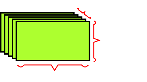
Images usually have three dimensions: height, width, and color channels. Grayscale images (black-and-white images, like our MNIST images) have only a single color channel. Colored images typically have three color channels: RGB (red, green, blue).
A batch of 500 grayscale images of size 256x256 could thus be stored in a rank-4 tensor of shape
(500, 256, 256, 1), whereas a batch of 500 colored images could be stored in a tensor a
shape (500, 256, 256, 3).
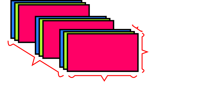
Video data is one of the few types of real-world data for which rank-5 tensors are used. A video can be simplified as a sequence of frames, each frame being a color image.
Each frame can be stored in a rank-3 tensor (height, width, color_channel).
A sequence of frames can be stored in a rank-4 tensor (frames, height, width, color_channel).
Therefore, a batch of videos can be stored in a rank-5 tensor of shape
(samples, frames, height, width, color_channel).
For instance, a 20-second, 1920x1080 video clip sampled at 10 frames per second would have 200 frames.
A batch of 5 such video clips would be stored in a tensor of shape (5, 200, 1920, 1080, 3).
That's a total of 6,220,800,000 values!
Similar to how computer programs can be reduced to a small set of binary operations (AND, OR, XOR, and so on), all transformations learned by deep neural networks can be reduced to a handful of tensor operations.
t1 + t2t1 - t2t1 * t2t1 / t2t1 ** t2t1 % t2t1 // t2tf.maximum(t1, t2)tf.minimum(t1, t2)tf.greater(t1, t2)tf.less(t1, t2)tf.greater_equal(t1, t2)tf.less_equal(t1, t2)tf.equal(t1, t2)tf.not_equal(t1, t2)More operations can be found in the tf.math module's API documentation here:
https://www.tensorflow.org/api_docs/python/tf/math
Element-wise operations are applied independently to each entry in the tensors being considered.
The relu, addition, and other operations listed above are all element-wise operations.
Recall in our initial example, we built our model by sequentially stacking Dense layers.
Each layer is a fully-connected layer with an activation function.
The first layer was a Dense layer with 512 nodes and activation function relu, like
so:
keras.layers.Dense(512, activation="relu")
From a Python standpoint, we could use for loops to implement a naive element-wise operation.
Take a look below at a naive Python implementation of the relu and addition operations.
def naive_relu(x):
    """Relu is the equivalent of `max(x, 0)`, or `np.maximum(x, 0.)` for NumPy tensors"""
    assert len(x.shape) == 2  # x is a rank-2 NumPy tensor
    x = x.copy()  # Avoid overwriting the input tensor
    for i in range(x.shape[0]):
        for j in range(x.shape[1]):
            x[i, j] = max(x[i, j], 0)
    return x

def naive_addition(x, y):
    """Naive implementation of `x+y`, where x and y are rank-2 NumPy tensors"""
    assert len(x.shape) == 2
    assert x.shape == y.shape
    x = x.copy()  # Avoid overwriting the input tensor
    for i in range(x.shape[0]):
        for j in range(x.shape[1]):
            x[i, j] += y[i, j]
    return x
In practice, when working with NumPy arrays, it's best to utilize NumPy's highly optimized, built-in functions rather than create naive implementations. NumPy's built-in functions are low-level, highly parallel, efficient tensor-manipulation routines that are typically implemented in C.
As seen below in a simple example, the built-in functions are over 100x faster than naive implementations. They're wicked fast!
import numpy as np
import time

x = np.random.random((20, 100))
y = np.random.random((20, 100))

t0 = time.time()

# This takes 0.02 seconds
for _ in range(1000):
    z = x + y  # Element-wise addition
    z = np.maximum(z, 0.)  # Element-wise relu
    print(f"Took: {time.time() - t0:.2f} seconds")

# This takes 2.45 seconds
for _ in range(1000):
    z = naive_addition(x, y)
    z = naive_relu(z)
    print(f"Took: {time.time() - t0:.2f} seconds")
Broadcasting is the process of performing element-wise operations on tensors with different shapes.
For example, consider two tensors t1 and t2 with shapes (2, 3) and
(3,).
The result of t1 + t2 is a tensor t3 of shape (2, 3) and the result of
t1 * t2 is a tensor t4 of shape (2, 3).
Below is the simplest example of multiplying tensor a by scalar b.
This example and the image following were taken directly from NumPy's documentation found here.
I encourage reading NumPy's documentation - at least read the NumPy fundamentals section - to gain a deep understanding of the topics discussed in this article.
>>> a = np.array([1.0, 2.0, 3.0])
>>> b = 2.0
>>> a * b

array([ 2.,  4.,  6.])
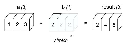
Simply put, the scalar b is stretched - the original scalar is copied - to become a tensor
of the same shape as a.
Getting a little more technical - broadcasting consists of two steps:
ndim of the
larger tensorValues from b are not actually copied - and b is not actually reshaped - as that would
be resource-intensive and computationally wasteful.
Rather, NumPy is smart enough to use the original scalar value without making copies so that broadcasting
operations are as memory and resource-efficient as possible.
import numpy as np
"""Example of how broadcasting "stretches" a vector into a matrix"""
x = np.random.random((28, 10))  # random matrix with shape (28, 10)
y = np.random.random((10,))     # random vector with shape (10,)

# add empty first axis to y, y.shape == (1, 10)
y = np.expand_dims(y, axis=0)
# repeat y 28 times along axis 0, shape == (28, 10)
y_stretched = np.concatenate([y] * 28, axis=0)

assert x.shape == y_stretched.shape
The stretching of scalar b qualifies the pair of variables for element-wise operations that take two
input tensors.
One of the most common and useful broadcasting applications include the tensor product or dot
product.
The tensor product, or dot product, is one of the most common tensor operations.
In NumPy, the tensor product is done using the np.dot function.
In mathematical notation, the dot product is denoted with a dot (⋅) symbol: z = x ⋅ y
# two random, 28-dimension vectors
x = np.random.random((28,))
y = np.random.random((28,))
z = np.dot(x, y)

# the (dot) product of two vectors is a scalar
assert isinstance(z, (int, float))
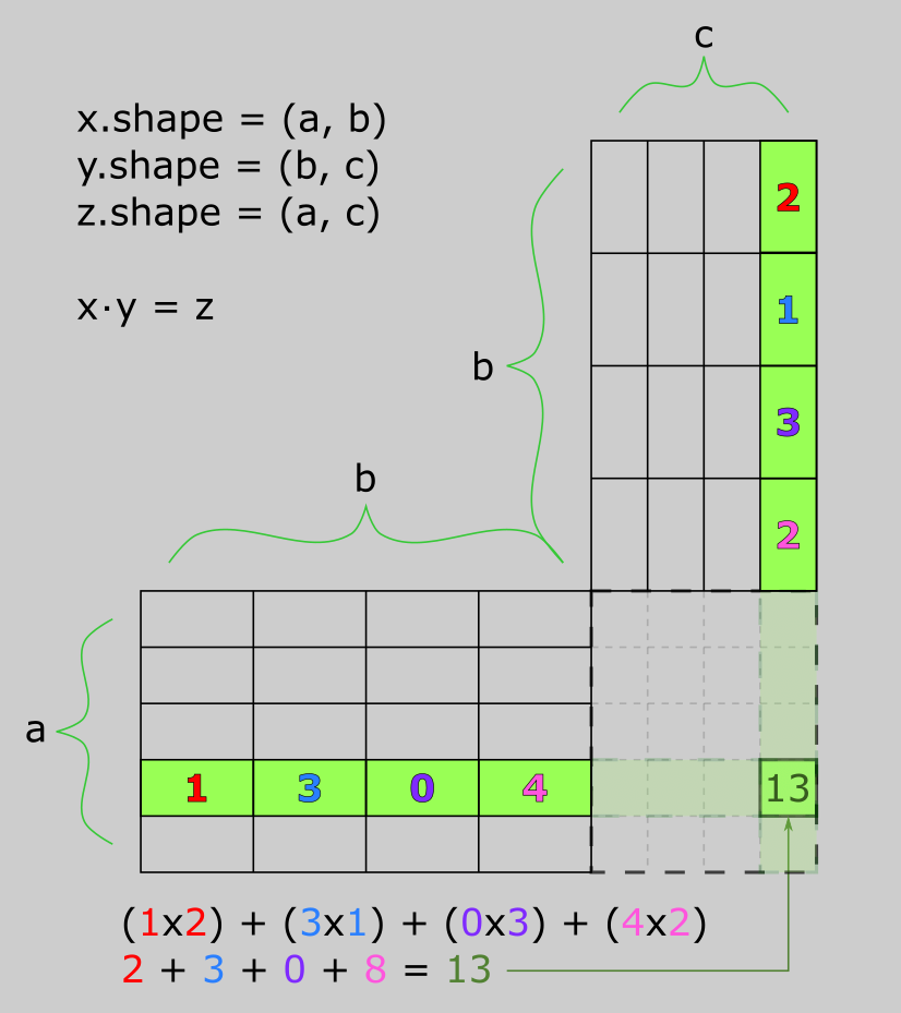
The most common application of the dot product in deep learning may be between two matrices:
dot(x, y).
The dot product between two matrices is only possible when x.shape[1] == y.shape[0].
The result is a matrix with shape (x.shape[0], y.shape[1]), where the coefficients are the vector
products between the rows of x and the columns of y.
More generally, we can take the dot product between higher-dimensional tensors following the same rules for shape compatibility as outlined earlier for the 2D case:
(a, b, c, d) ⋅ (d,)   -> (a, b, c)
(a, b, c, d) ⋅ (d, e) -> (a, b, c, e)
A third tensor operation that's crucial to deep learning is tensor reshaping. We first encountered tensor reshaping earlier in the chapter when we processed input images for our neural network.
train_images = train_images.reshape((6000, 28*28))
Reshaping is the rearranging of a tensor's columns and rows. Expectedly, the result is a tensor with the same number of elements as the original tensor, but with a new shape. Consider the following example:
>>> x = np.array([[1, 2, 3], [4, 5, 6]])
>>> x.shape
(2, 3)
>>> y = x.reshape((3, 2))
>>> y
array([[1, 2],
       [3, 4],
       [5, 6]])
>>> y.shape
(3, 2)
>>> z = y.reshape((6, 1))
>>> z
array([[1], [2], [3], [4], [5], [6]])
A common reshaping operation is the flattening of a tensor. The flattening operation is simply the concatenation of all the elements of a tensor into a single vector.
>>> x = np.array([[1, 2, 3], [4, 5, 6]])
>>> x.flatten()
array([1, 2, 3, 4, 5, 6])
A special case of the reshaping operation is the transposing of a tensor. The transpose operation is simply the reverse of the reshaping operation.
>>> x = np.array([[1, 2, 3], [4, 5, 6]])
>>> x.shape
(2, 3)
>>> y = x.transpose()
>>> y.shape
(2, 3)
>>> y
array([[1, 4], [2, 5], [3, 6]])

>>> x = np.zeros((200, 3))
>>> y = x.transpose()
>>> y.shape
(3, 200)
A seemingly useless case of tensor reshaping - generated by CoPilot - is when the new shape is a singleton. For example, we can reshape a vector to a scalar:
>>> x = np.array([1, 2, 3])
>>> x.shape
(3,)
>>> y = x.reshape(())
>>> y
1
>>> y.shape
()
The book goes into deep detail about the geometric interpretations of deep learning and tensors operations.
François compares tensor operations to vector/matrix addition, translation, rotation, scaling, and other geometric operations. I believe these are fundamental concepts for understanding how data transformations are performed in neural networks as they provide a different perspective on the way data is processed. However, I will not be covering these concepts in this article because they diverge from the high-level concepts I wish to cover. I recommend reading the book's chapter on geometric interpretations of tensor operations.
Each neural layer from our first model example transforms its input data as follows:
output = relu(dot(input, W) + b)
In this expression, W and b are tensors from the layer attributes - W is
the weight matrix and b is the bias vector.
These variables are also called the trainable parameters (kernel and bias
attributes, respectively) of the layer.
The weights contain the information learned by the model from exposure to training data.
Upon initializing the model, the weights are randomly initialized - filled with random values. What comes next is to gradually update the weights based on a feedback signal from the loss function. The gradual adjustment of weights, also called training, is how the neural networks learn. Training is what machine learning is all about!
The model trains in what's called a training loop. At a high level, the following steps are repeated until the loss function converges:
x, and corresponding target labels, y_truex - a step called the forward pass - to obtain predictions,
y_pred
y_true and
y_pred
Step 1 is easy: we load our dataset (images, tabular data, etc.) and their corresponding labels. Steps 2 and 3 are a handful of tensor operations and basic mathematics. Step 4, however, is the most difficult part. We will cover the high-level details of step 4 in the following gradient descent and backpropagation sections.
NOTE: Assumptions
This section assumes that you are familiar with tensor operations and the concept of derivatives in calculus. Below are some helpful rules to keep in mind:
- Gradients can be interpreted as the direction of the steepest ascent of some function with respect to some variable.
- Given a differential function, it's possible to find its minimum when the derivative is zero.
- For a neural network, the minimum can be found by solving for
grad(f(W), W) = 0orgrad(loss_score, W) = 0using gradient descent.
The derivative of a tensor operation (or tensor function) is called a gradient.
The concept of derivation can be applied to any function, as long as the surfaces they describe are continuous
and smooth.
For example, the tensor operations used in our model - such as relu, dot, addition,
etc. - are all continuous and smooth.
All of the functions used in our models (such as dot or +) transform their input
smoothly and continuously.
Therefore, we can derive the gradient of all the tensor operations used in our model and use it to update the
weights of the model.
For instance, if we look at z = x + y, we can determine that a small change in x will
not change z much, but a large change in x will change z much more.
Furthermore, if we know the direction of the change in x, we can infer the direction of the change
in z.
In mathematics, we called these differentiable functions.
We can use the inferred direction of change to update the model's weight in a way that will incrementally reduce
the loss during training.
Mathematically, the gradient of a function represents the curvature of the multidimensional surface described by the function. Simply put, gradients characterize how the output of the function varies when its input parameters vary.
Gradient descent is a common technique for optimizing neural networks by nudging the parameters of a neural
network towards the minimum of the loss function.
Essentially, it's the process for solving the equation grad(f(W), W) = 0.
It's the key to figuring out what combination of weights can output the lowest loss.
Tying gradients back to weight updates and loss scores, the gradient can be used to move the weights of the model towards the minimum of the loss function. The weights are moved opposite to the direction of the gradient.
Why are weights moved in the opposite direction of the gradient?
The gradient - such as grad(loss_score, W0) - can be interpreted as the direction of
steepest ascent of loss_value = f(W) with respect to W0, where
f is the loss function.
Intuitively, moving W1 in the opposite direction of the steepest ascent
(grad(loss_score, W0) will move the weights closer to a lower point of the curve - hence the name,
gradient descent.
When done incrementally during training, we see that the weights converge to the minimum of the loss function.
Let's update the training loop process from above to include gradient descent:
x, and corresponding target labels, y_truex - a step called the forward pass - to obtain predictions,
y_pred
y_true and
y_pred
W -= learning_rate * gradient - thus reducing the loss on the batch.
learning_rate) would be a scalar responsible for modulating
the magnitude of the descent - or how big of a step the weights are moved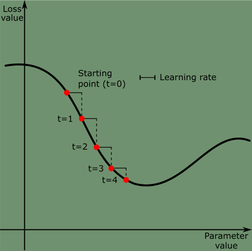
It's important to pick a reasonable value for the learning_rate.
If it's too small, the descent down the curve will take many iterations and may get stuck in a local minimum.
If it's too large, the updates will be too big and may take you to completely random locations on the curve.
There exist multiple variants of gradient descent. These variants are known as optimizers or optimization algorithms.
The variant used above is called stochastic gradient descent - more specifically, mini-batch stochastic gradient descent (SGD). SGD is a simple variant that looks only at the current value of the gradients.
Other variants - such as Adagrad, RMSprop, and so on - differ by taking into account previous weight updates when computing the next weight update. This is an important concept called momentum.
Momentum is the process of using previous weight updates to compute the next weight update. It addresses two issues with SGD:

Around a specific point in the figure beside, we can see there is a local minimum where moving left results in the loss increasing, but so does moving right. If the parameters were optimized via SGD with a small learning rate, the loss would get stuck at the local minimum instead of the global minimum.
The concept of momentum is inspired by physics - such as a small ball rolling down the loss curve. If the ball has enough momentum, it won't get stuck in the local minimum.
Momentum is implemented by moving the ball at each step based not only on the current slope value (current
acceleration) but also on the current velocity (resulting from pass acceleration).
This means updating the parameter w based not only on the current gradient value but also on
previous parameter updates.
Take a look at this naive implementation:
past_velocity = 0
momentum = 0.1
while loss > 0.01:
    w, loss, gradient = get_model_parameters()
    velocity = past_velocity * momentum - learning_rate * gradient
    w = w + momentum * velocity - learning_rate * gradient
    past_velocity = velocity
    update_model_parameters(w)
A neural network consists of many tensor operations chained together: dot, relu,
softmax, and +.
Each operation has a simple, known derivative.
Backpropagation is the process of finding the derivative of the loss function with respect to the weights and
biases of a neural network.
Mathematically, Calculus tells us that a chain of functions can be derived using the chain rule.
Consider the two functions f and g, and the composed fg such that
fg(x) = f(g(x)):
def fg(x):
    x1 = g(x)
    y = f(x1)
    return y
Mathematically, the chain rule states that grad(y, x) == grad(y, x1) * grad(x1, x).
In English, the chain rule states that the derivative of fg with respect to x is the
derivative of f with respect to x1 times the derivative of g with respect
to x.
This enables us to compute the derivative of fg as long as we know the derivatives of
f and g.
Let's increase the size of the composed function to further understand why it's called the chain rule:
def fghj(x):
    x1 = j(x)
    x2 = h(x1)
    x3 = g(x2)
    y = f(x3)
    return y
Then the chain rule states that
grad(y, x) == grad(y, x3) * grad(x3, x2) * grad(x2, x1) * grad(x1, x).
Let's dive deeper into the algorithm using computation graphs.
Using the backpropagation algorithm, we can get the gradient of the loss with respect to the weights and biases
of the network.
Mathematically, we're solving the following equation: grad(loss_score, w) = 0.
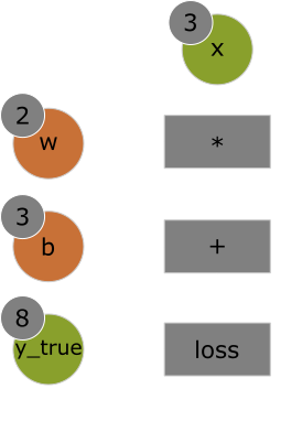
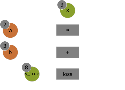
Computation graphs are simple data structures that represent operations as data.
It's a directed acyclic graph of operations - in our case, tensor operations.
The image below is an example of a computation graph of a forward pass with input x and operations
*, +, and loss, where loss is our loss function
loss_score = abs(y_true - x2).
The forward pass has input x = 3 with parameters w = 2 and b = 3,
resulting in loss_score = 1.
Simple enough to read a computation graph, right? Let's look at the computation graph of a backward pass to learn how to compute the gradients. Given the backward pass graph, we can compute the following gradients:
grad(loss_score, x2) = 1, because as x2 varies by an amount epsilon, the
loss_score = abs(8 - x2) changes by the same amount epsilon
grad(x2, x1) = 1, because as x1 varies by an amount epsilon, the
x2 = x1 + b = x1 + 1 changes by the same amount epsilon
grad(x2, b) = 1, because as b varies by an amount epsilon, the
x2 = x1 + b = 6 + b changes by the same amount epsilon
grad(x1, w) = 3, because as w varies by an amount epsilon, the
x1 = w * x = 3 * x changes by 3 * epsilon
The chain rule says that we can obtain the derivative of a node with respect to another node by multiplying
the derivatives for each edge along the path linking the two nodes.
Therefore, we can compute the gradient of the loss_score with respect to the weights
(grad(loss_score, w)) using the chain rule.
For instance, the figure below shows the path from loss_score to w.
The path produces the following gradient calculation:
grad(loss_score, w) = grad(loss_score, x2) * grad(x2, x1) * grad(x1, w).
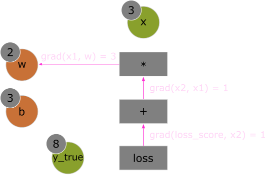
By applying the chain rule to our graph, we obtain what we were looking for:
grad(loss_score, w) = 1 * 1 * 3 = 3grad(loss_score, b) = 1 * 1 * 1 = 1That's the backpropagation algorithm using a simple computation graph example. The algorithm starts with the final loss score and works backward from the bottom layer to the top layers, computing the contribution of each parameter to the loss score.
Now imagine a neural network with hundreds of layers and parameters. Calculating the gradient by hand would be tedious, error-prone, and time-consuming. That's why TensorFlow provides a way to compute the gradients for us through automatic differentiation.
The API through used to leverage TensorFlow's automatic differentiation is the GradientTape.
It's a Python context that will "record" tensor operations executed within the context in the form of
computation graphs.
The computation graphs are used to retrieve the gradient of any output with respect to any variable or set of
variables (instances of the tf.Variable class).
NOTE:
tf.VariableclassThe
tf.Variableclass is simply a container that holds a mutable tensor. For instance, the weights of a neural network are stored intf.Variableinstances. Read more abouttf.Variableclass in the TensorFlow documentation.
import tensorflow as tf
# Initialize a variable with a scalar value of 3
x = tf.Variable(3.0)
# Open a GradientTape context, or scope
with tf.GradientTape() as tape:
    # Apply some operations within the context to our variable x
    y = 5 * x + 2
# Use the tape to retrieve the gradient of y with respect to x
grad_of_y_wrt_x = tape.gradient(y, x)
# The gradient of y with respect to x is 5
print(grad_of_y_wrt_x.numpy())
The GradientTape works with tensor operations and lists of variables as well:
# Initialize a Variable of shape (2, 2) with random initial values
x = tf.Variable(tf.random.uniform((2, 2)))
with tf.GradientTape() as tape:
    # Apply tensor operations within the context to our variable x
    y = 5 * x + 2
grad_of_y_wrt_x = tape.gradient(y, x)
# The gradient of y with respect to x is [[5, 5], [5, 5]
# Tensor of shape (2, 2) - just like x - describing the curvature of
# y = 5 * x + 2 around randomly-initialized x
print(grad_of_y_wrt_x.numpy())

W = tf.Variable(tf.random.uniform((2, 2)))
b = tf.Variable(tf.zeros(2,))
x = tf.random.uniform((2, 2))
with tf.GradientTape() as tape:
    # `tf.matmul()` is the dot product equivalent in TensorFlow, or @ in numpy
    y = tf.matmul(x, W) + b

# List of two tensors with the same shapes as W and b, respectively
grad_of_y_wrt_W_and_b = tape.gradient(y, [W, b])
grad_of_y_wrt_W = grad_of_y_wrt_W_and_b[0]
grad_of_y_wrt_b = grad_of_y_wrt_W_and_b[1]

print(grad_of_y_wrt_W.numpy())
print(grad_of_y_wrt_b.numpy())
More information regarding the GradientTape can be found in the TensorFlow documentation and Chapter 3
of Deep Learning with Python.
We should now have a general understanding of what's going on behind the scenes in a neural network. What was previously a mysterious black box has turned into a clearer picture seen below: the model, composed of sequential layers, maps the input data to predictions. The loss function then compares the predictions to the target values, producing a loss value: a measure of how well the model's predictions match what was expected. The optimizer uses this loss value to update the model's weights.
Now we understand that the input images are stored in NumPy tensors.
Before training the model, the input images - training and testing images - were pre-processed: training tensors
were converted to type float32 and reshaped to shape (60000, 28*28) from
(60000, 28, 28), and testing tensors were similarly reformatted and reshaped
(10000, 28*28) from (10000, 28, 28).
(train_images, train_labels), (test_images, test_labels) = mnist.load_data()
train_images = train_images.reshape((60000, 28 * 28))
train_images = train_images.astype("float32") / 255
test_images = test_images.reshape((10000, 28 * 28))
test_images = test_images.astype("float32") / 255
Recall that our two-layer neural network model was created like so:
from tensorflow import keras
from tensorflow.keras import layers
model = keras.Sequential([
    layers.Dense(512, activation="relu"),
    layers.Dense(10, activation="softmax")
])
We now understand that this model consists of a chain of two Dense layers.
Each layer performs simple tensor operations to the input data, further refining the data to more useful data
representations.
These layers incorporate the usage of layer weight tensors. Weight tensors, which are attributes of the layers, are where the knowledge of the model persists.
This was the model-compilation step:
model.compile(optimizer="rmsprop",
              loss="sparse_categorical_crossentropy",
              metrics=["accuracy"])
We understand that sparse_categorical_crossentropy is the loss function that's used to calculate the
loss score.
The loss score is used as a feedback signal for learning the weight tensors.
During the training phase, the training loop will attempt to minimize the loss score.
The reduction of the loss happens via mini-batch stochastic (random) gradient descent.
The exact rules and specifications of loss reduction are defined by the rmsprop optimizer passed as
the model's first argument.
Finally, this was the model's training loop:
model.fit(train_images, train_labels, epochs=5, batch_size=128)
Fitting the model to the training data is simple: the model will iterate on the training data in a mini-batch of 128 samples, 5 times over. Each iteration over the entire training dataset is called an epoch. Given that there are 60000 training images, there are a total of 60000/128 (~469, or 500) mini-batches.
For each mini-batch, the model will compute the gradient of the loss with regard to the weights. Using the Backpropagation algorithm (which derives from the chain rule in calculus), the optimizer moves the weights in the direction that will reduce the value of the loss for this batch.
And that's it! It sounds complicated when all the keywords are used, but we firmly understand that it's simply matrix multiplication, addition, subtraction, and derivatives.
Tensors form the foundation of modern machine learning systems. They come in various flavors of
rank, shape, and dtype.
We can manipulate numerical tensors via tensor operations: addition, tensor product, or element-wise multiplication. In general, everything in deep learning is comparable to a geometric transformation.
Deep learning models consist of sequences of simple tensor operations, parameterized by weights, which are tensors themselves. The weights of a model are where the model's "knowledge" is stored.
Learning means finding a set of values for the model's weights such that the loss score is minimized for a given batch of training data samples.
Learning happens by drawing random batches of data samples and their targets and computing the gradient of the model parameters with respect to the batch's loss score. The model's parameters are then moved - the magnitude of which is determined by the learning rate - in the opposite direction from the gradient. This is called mini-batch stochastic gradient descent.
The entire learning process is made possible by the fact that all tensor operations in neural networks are differentiable, making it possible to apply the chain rule of derivation. The chain rule of derivation allows us to find the gradient function mapping the current parameters and current batch of data to a gradient value. This is called backpropagation.
Two key concepts we'll see frequently in future chapters are loss and optimizers.