January 25, 2022
Minimax search is a fundamental depth-first search algorithm used in Artificial Intelligence, decision theory, game theory, and statistics. The purpose of minimax search is to minimize the maximum loss in a worst-case scenario - or, simply put, figure out the best action to pursue in a worst-case scenario.
This algorithm can be implemented in n-player perfect information games but is most commonly implemented in 2-player zero-sum games such as Checkers, Chess, Connect 4, Mancala, Tic-Tac-Toe, etc. Zero-sum games are simplified as games where whatever (value/utility) one player wins and, the other player loses.
Perfect information games are games where every player knows the results of all previous moves. In games of perfect information, there is at least one "best" way to play for each player. The "best" way to play can be obtained by searching into future moves using and evaluating the game states with search algorithms such as minimax. Moreover, the best strategy does not necessarily allow one to win but will minimize the losses3.
In this article, we'll discuss what minimax search is, the related vocabulary, search tree structure, search process, alpha-beta pruning, and, finally, implement minimax with and without alpha-beta pruning in mancala.
Let's familiarize ourselves with minimax-related variables and keywords before we implement minimax searches.
| Keyword | Variable | Definition |
|---|---|---|
| Player/Maximizer | pmax1 | Maximizes their action's value - or minimizes the maximum loss - in a worst-case scenario |
| Opponent/Minimizer | pmin | Minimizes the value of the player's (pmax's) maximum gain |
| Heuristic value | v2 |
Value of the player's action - or current game state - obtained by an evaluation function. Larger numbers are more beneficial for pmax, whereas smaller numbers are more beneficial for pmin. |
| Branching factor | b |
How many actions the player has available |
| Depth | d |
How deep into the tree - or how many moves ahead - the algorithm will search |
Suppose we're playing a 2-player turn-based game where each player has a choice between two actions per turn.
The branching factor, b, will be equal to 2.
We'll configure the algorithm to search to a depth of 3 - that is, we'll consider the player's possible moves,
the opponent's responses, and the player's responses to the opponent's responses - which will set the variable
d equal to 3.
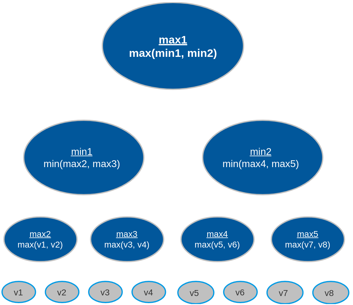
Given the variables b=2 and d=3, the algorithm will generate the following tree
structure:
The number of heuristic evaluations - also called terminal nodes or leaf nodes, seen in the figure as v1-v8 - completed in a minimax search tree is denoted by: bd. It's important to notice that the size of the search tree increases exponentially based on how deep the algorithm searches and how large the branching factor is.
We have a mere 23 (8) heuristics evaluations in the tree above when looking 3 moves ahead. However, the tree represents an arbitrary game for which there are only two possible actions per turn.
Consider chess, where the branching factor (possible moves) is exactly 20 for opening moves and about 35 for the
remainder of the game4.
If we re-configured our minimax algorithm's branching factor (b) to reflect the number of possible
moves in chess, we would have to perform roughly 353 (42,875) heuristic evaluations.
And that's only looking 3 moves ahead!
The last thing to consider about these trees is that the branching factor is not always uniform. Just because there are two possible moves this turn, it doesn't mean there will be two possible moves next turn. Perhaps there is only one possible move next turn or you may have reached a terminal state where there are no possible moves; you've won or lost.
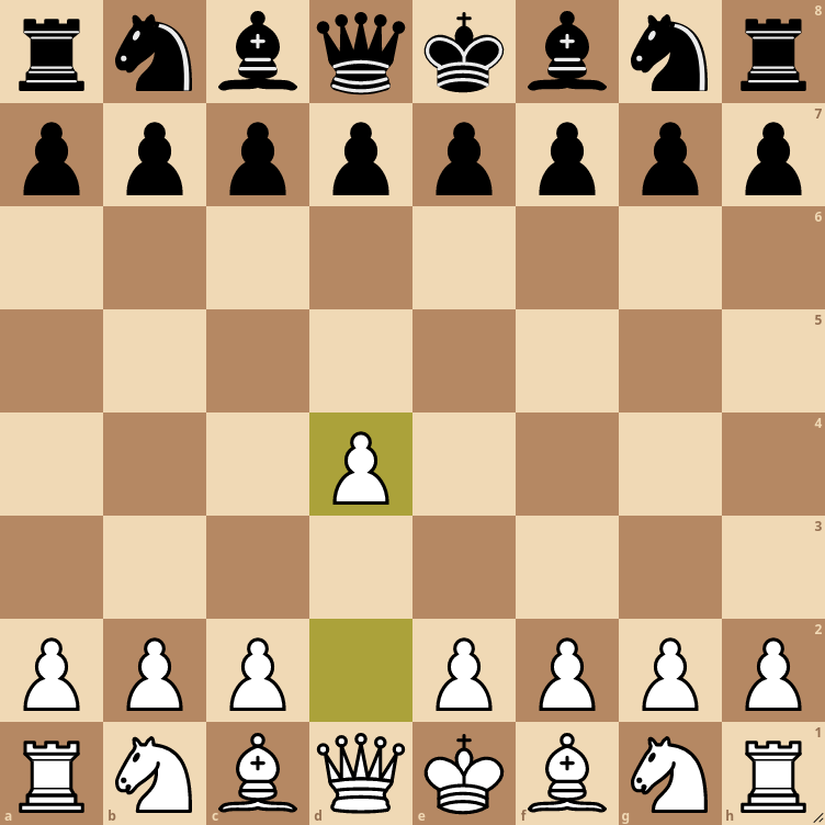
Looking at chess again... there are 20 possible opening moves. After the first move, and depending on which piece is moved, there can be anywhere from 20 to 29 moves. The opening move below allows for 29 possible moves on white's next turn - or 28 possible moves if black moves their pawn to d5.
Recall that minimax search is a depth-first search algorithm; it starts at the root node and travels as deep as possible through each branch before backtracking to the top of the tree. The depth-first search is complete once all nodes have been visited.
Depth-first search animation
Minimax evaluates all terminal nodes at the maximum search depth d and then begins the search
process.
The non-terminal nodes' values are determined by the minimizer/maximizer's choices of the descendent leaf nodes.
Referring back to the minimax tree, the search process begins as follows for a tree with depth 3:
max2 picks the maximum value between v1 and v2min1 and calculates the terminal node values of
v3 and v4max3 picks the maximum value between v3 and v4min1 picks the minimum value between max2 and
max3
max4(v5, v6), max5(v7, v8), and min2(max4, max5)max1 (root node) picks the maximum value between min1 and
min2
The gist of minimax is that the minimizer and maximizer alternate picking their most optimal value for every level of the tree. Who picks first depends on how deep the tree is, but it's guaranteed that the maximizer picks last because they are the root node and the main player.
When the search completes, the root node will contain the player's maximum gain in a worst-case scenario,
assuming the opponent is always playing their best move.
Minimax with deep searches (large d value) are not optimal against opponents with random actions
because the algorithm assumes the opponent is competent and playing optimal moves.
One last thing to consider is that the algorithm's search time drastically increases for complex games with a
large branching factor b - also called action spaces - such as chess.
The algorithm visits every node - every possible action - before choosing an optimal action.
So the larger and deeper the tree, the longer the search algorithm takes to find the most optimal value.
The search time of large trees can be dramatically reduced by applying an optimization called alpha-beta pruning.
Alpha-beta pruning is an optimization technique for the minimax search algorithm. The optimization greatly reduces search times by preventing minimax from visiting and evaluating unnecessary nodes.
Recall that the number of nodes visited by minimax is exponential (bd). In best-case scenarios, alpha-beta pruning reduces the exponent in half, thus considerably improving search times. But how does alpha-beta pruning optimize search times?
The pruning process cuts off leaves - or entire sub-trees - in the game tree which need not be searched because a better move already exists. It's easy to think that the algorithm may prune the most optimal action; however, alpha-beta pruning will return the same action as minimax, only much faster.
The optimization technique adds two new terms to our minimax vocabulary: alpha (α) and beta
(β)
| Keyword | Variable | Definition |
|---|---|---|
| Alpha | α |
The best action (highest value) pmax can guarantee at the current tree depth or above. Initial value is -∞. |
| Beta | β |
The best action (lowest value) the pmin can guarantee at the current tree depth or above. Initial value is +∞. |
Before diving into the pruning process, we need to understand the principles of alpha-beta:
αβα and β values are passed down only to the child nodes; not to the parent nodes
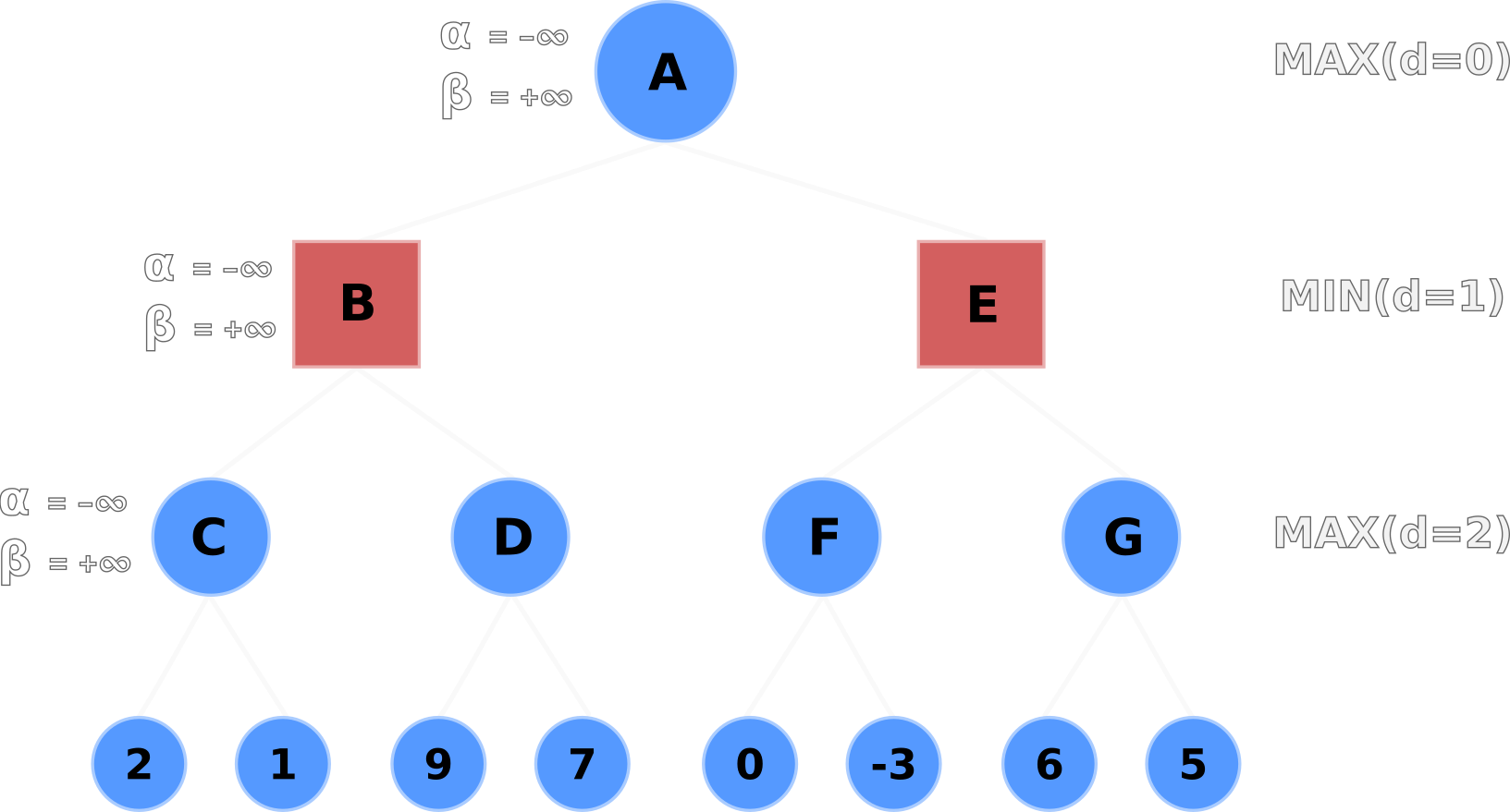
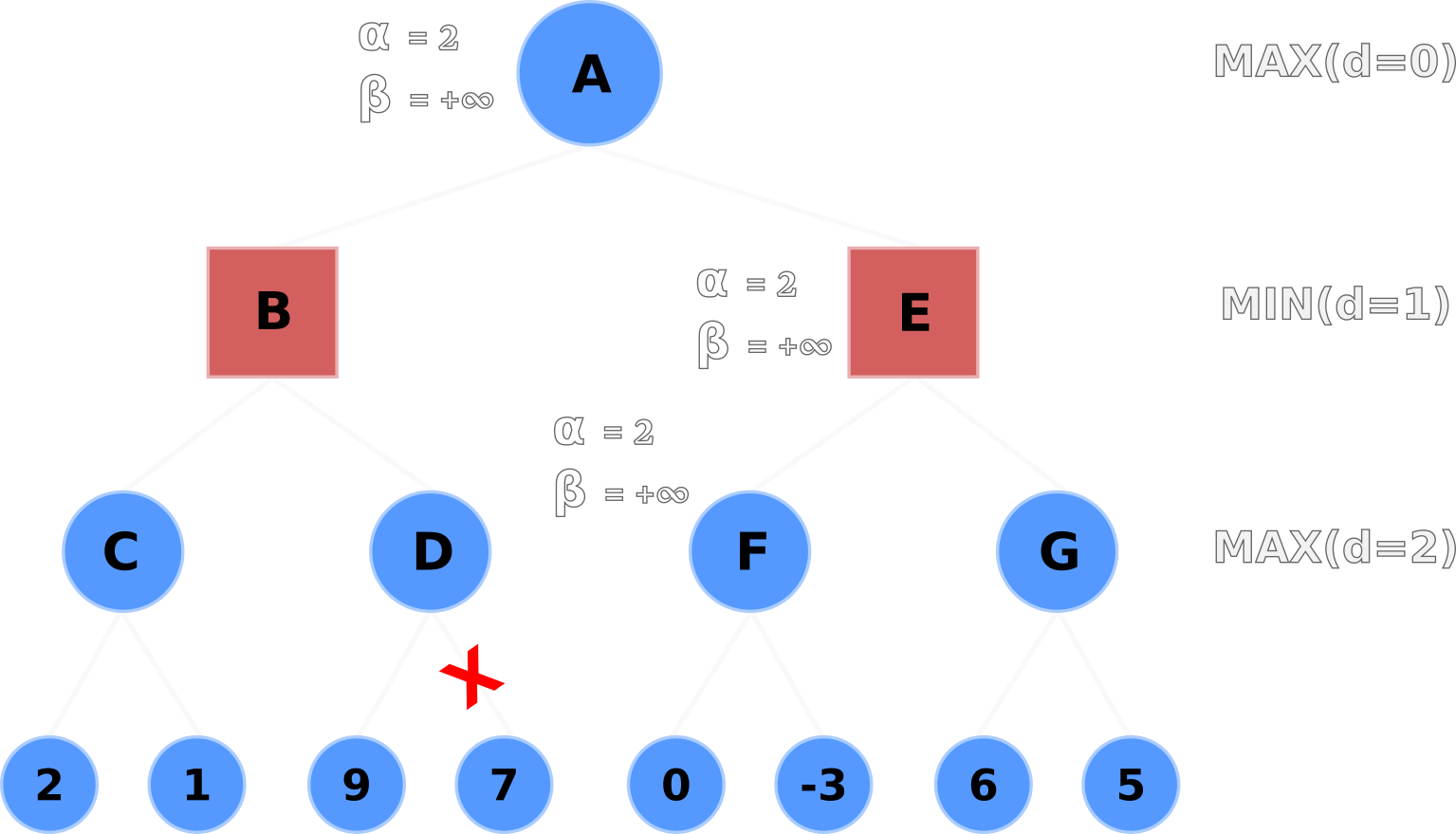
α>=βLet's now walk through the alpha-beta pruning process. In the following figures, Nodes A, C, D, F, G are the maximizers, and Nodes B, E are the minimizers.
The default α and β values are propagated from A to its children B and C.
Node C evaluates its left-hand terminal node (2) and compares it to the current α value.
If the terminal node's value is greater than the current α value - e.g. max(2, -∞) - then Node C
updates α with the terminal node's value.
Node C's node and α values are now equal to 2 because 2 is greater than -∞.
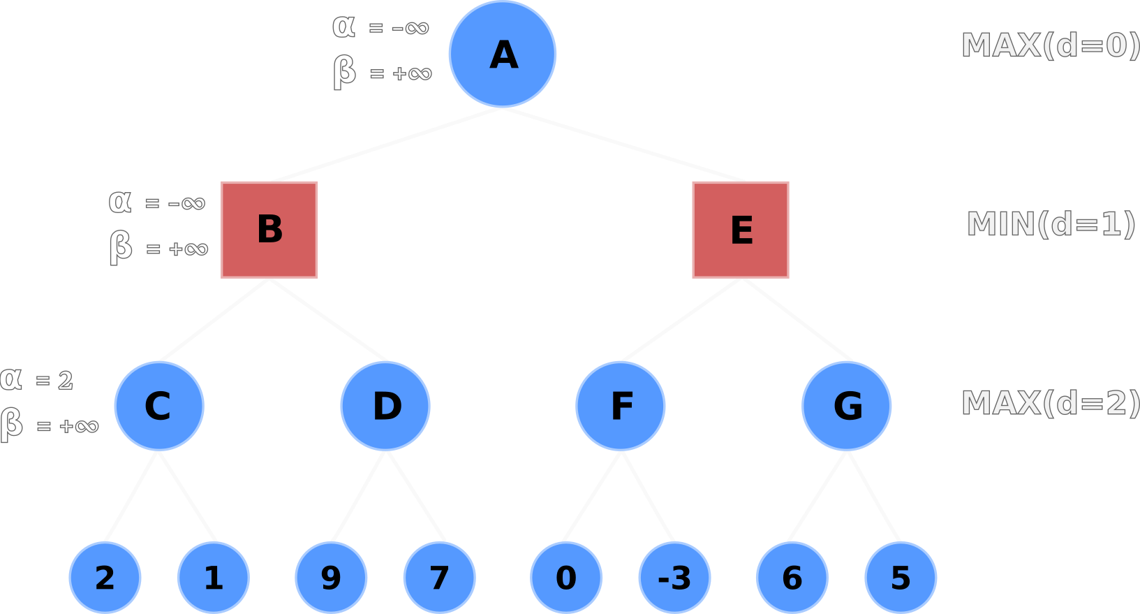
α valuesNode C then evaluates its right-hand terminal node.
The right-hand node's value (1) is less than α (2) and less than Node C's current value (2), so
nothing is updated.
Node C's value is backtracked upwards; Node B's value is set to 2.
Node B then compares its β value (+∞) to its current node value (2) and updates β if
the current node value is less than β - e.g. min(2, +∞).
Node B's β value is now set to 2 and propagated downwards to Node D's β value.
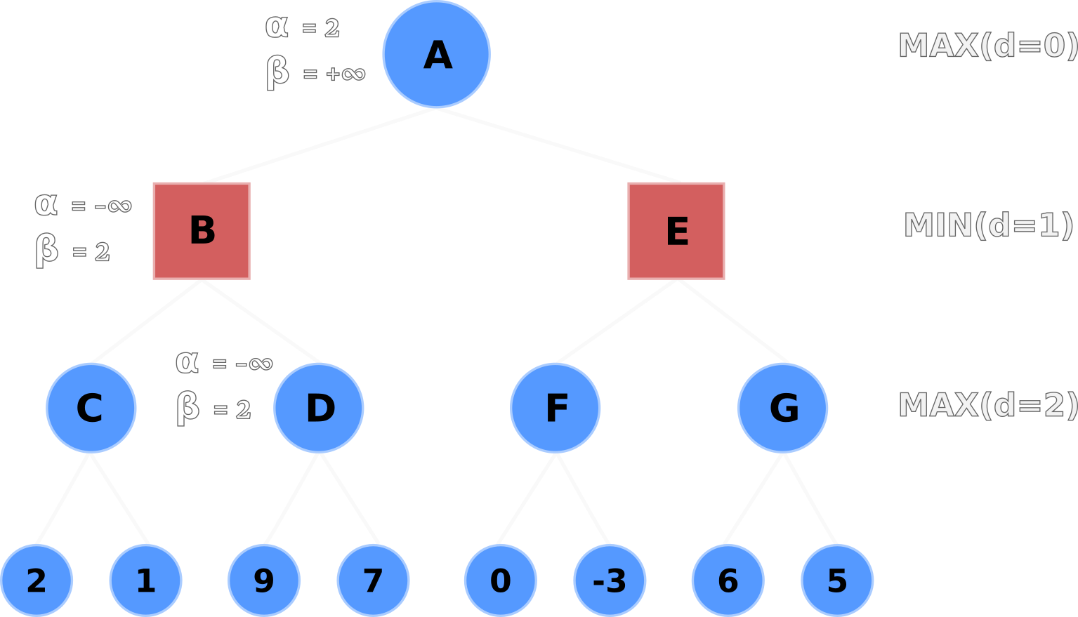
β, values following C's backtrack, then propogates its
β to D
Node D evaluates the left-hand node and updates its node and α values to 9.
Here's the important part: Node D's α value is now greater than its β
value, so it no longer has to evaluate the remaining nodes.
The right-hand node is pruned, thus saving the algorithm from evaluating the heuristic value of one node so far.
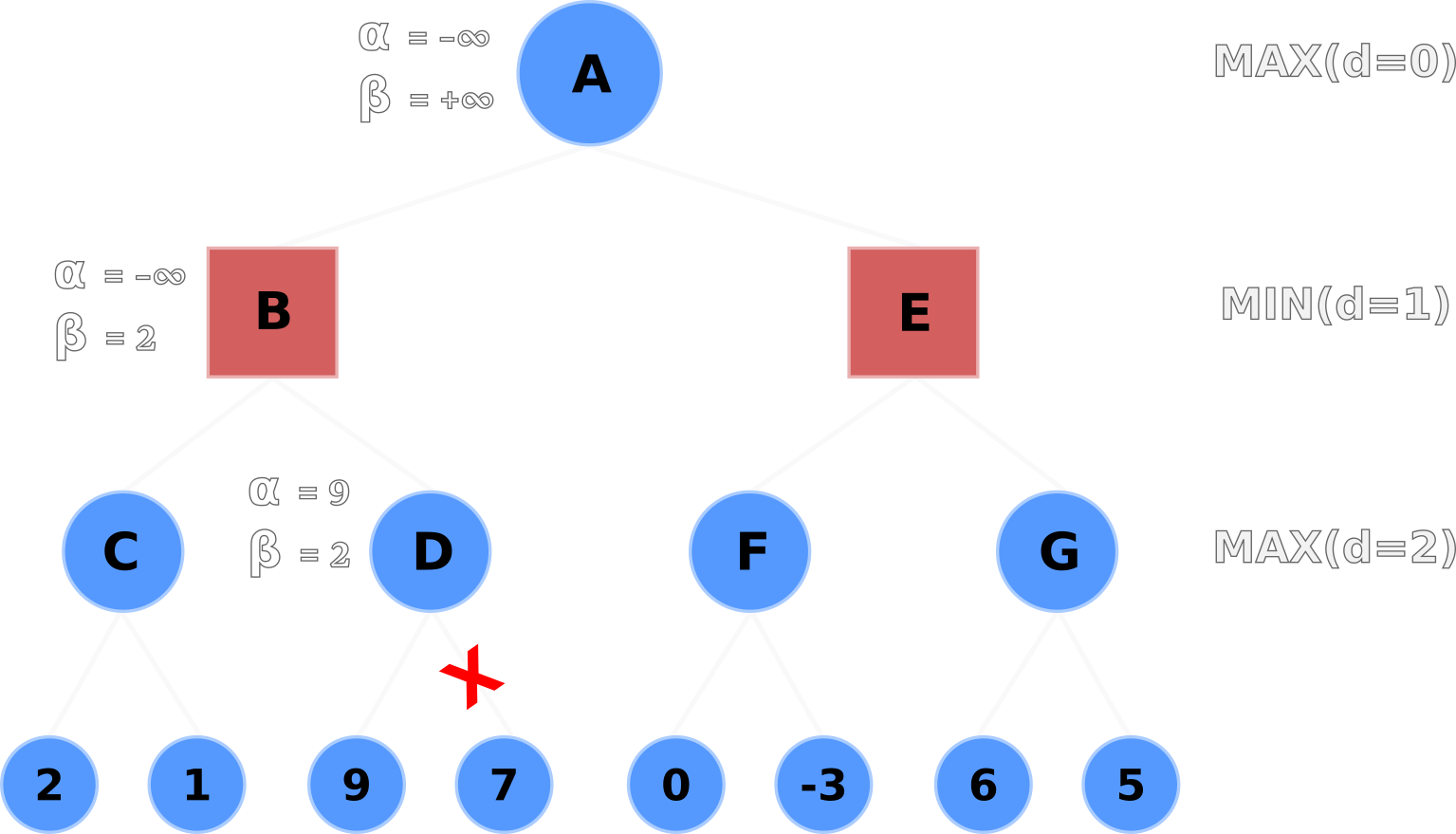
α value because it's a
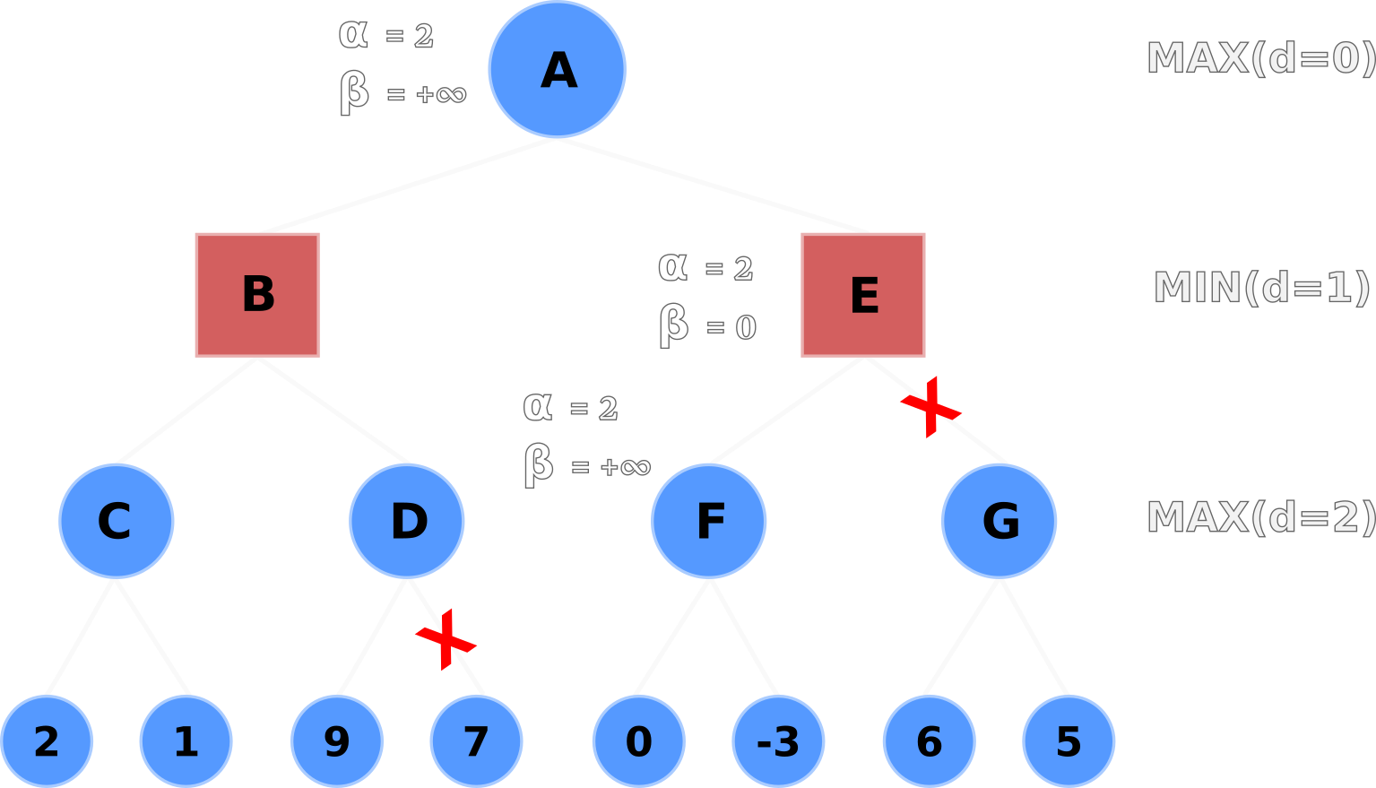
pointless computationNode D backtracks its node value to Node B.
Node B selects the minimum value from C and D with min(2, 9), and selects 2.
Node B then backtracks its node value to Node A, and Node A updates its node and α values to 2
after evaluating max(2, -∞).

α values following B's backtrackNode A propagates its alpha-beta values (α=2, β=+∞) down to Nodes E and F.
Node F evaluates its left-hand terminal node (0) and selects 0 for its node value, but does not update the
α value because max(0, 2) is still 2.
Node F then evaluates the right-hand node but doesn't update its node or α value because -3 is less
than 0 and 2.
α value to children Nodes E and FNode F backtracks its node value up to Node E, where E will update its β value with 0 after
evaluating min(0, +∞).
Now E's alpha-beta values are (α=2, β=0).
Here's another important part: Node E's α value is greater than its β
value, so it prunes the entire sub-tree of Node G.
Thus saving the algorithm from two more node evaluations, for a total of three fewer heuristic evaluations
overall.
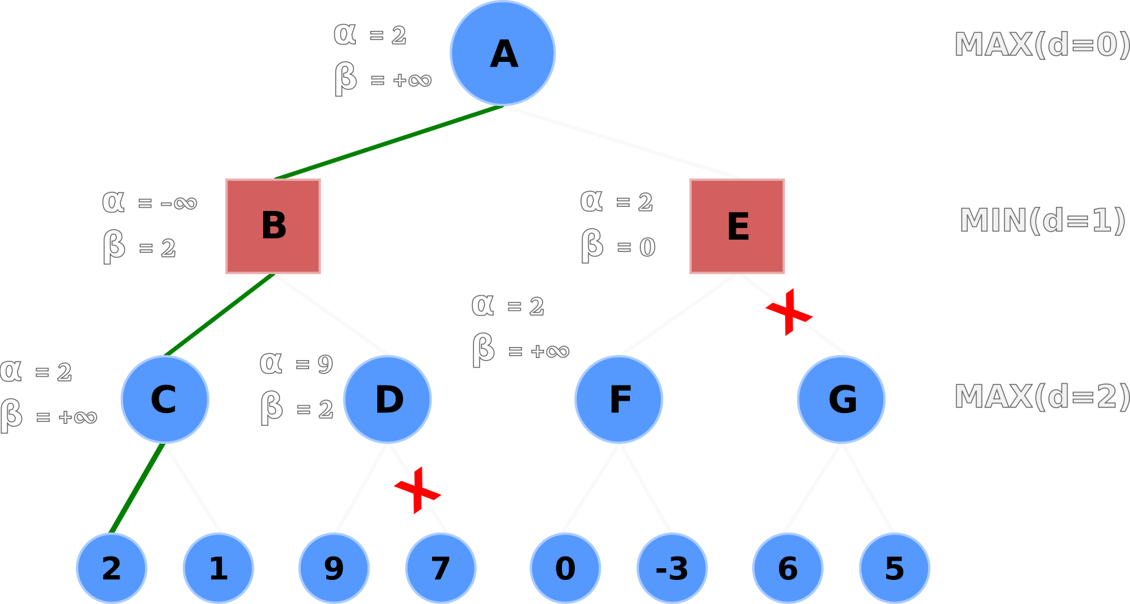
α value is greater than its
β value
Node E backtracks its node value of 0 up to Node A where Node A will take the max(B, E) or max(2, 0).
Of course Node A will select 2. And that's how we can find the player's most optimal action in a worst-case scenario using minimax with alpha-beta pruning!
The order in which nodes are examined directly affects alpha-beta pruning's effectiveness. There are two types of node orderings to be conscious of before creating a minimax game tree:
How can we prevent the worst ordering?
Order moves from best to worst using domain knowledge so the best move resides on/near the left-most terminal node.
In Chess, for instance, certain actions are more valuable than others: winning captures, promotions, equal captures, non-captures6. If we wanted to maximize the alpha-beta pruning process on a Chess game tree, we'd order the nodes from most valuable to least valuable - aka an ideal ordering.
Mancala is a 2-player turn-based board game. Each player has 6 pits with 4 seeds/stones along with 1 mancala (store) at the end of the board.
Players take turns picking up all the seeds from one of their 6 pits and placing them one by one until they're holding no seeds. Stones are placed counterclockwise into pits and in the player's mancala at the end of the board. Players must not place seeds in their opponent's mancala.
There are two exceptions for when a player can go again, or re-turn:
Lastly, there is a capture rule: If the last stone in the player's hand lands in an empty pit on their side of the board, and the adjacent pit on the opponent's side contains 1+ seeds, the player may capture all seeds from both pits and place them in their mancala.
The player's goal is to have more seeds in their mancala than their opponent.
The game ends on either of two conditions:
Please watch this 3-minute video if the explanation above wasn't clear.
I wrote a simple, CLI Mancala game simulator in Python. The code can be found on my GitHub repo. An example of the simulator can be seen below.
The top-most row is the indices of Player 1's pits. The following row is Player 1's pits initialized with 4 seeds. The left-most number is Player 1's mancala index, 13. The number immediately to the right of Player 1's mancala is his/her score. Everything else is Player 2's indices, pits, or mancala.
   0   1   2   3   4   5
   |===============================|
   |---| 4 | 4 | 4 | 4 | 4 | 4 |---|
  13 | 0 |=======================| 0 | 6
   |---| 4 | 4 | 4 | 4 | 4 | 4 |---|
   |===============================|
   12  11  10  9   8   7

Player 1's Turn! Choose a number in range [0, 1, 2, 3, 4, 5]
    Player 1 selected pit 1: 4 seeds (+1, 0, 0)

   0   1   2   3   4   5
   |===============================|
   |---| 5 | 0 | 4 | 4 | 4 | 4 |---|
  13 | 1 |=======================| 0 | 6
   |---| 5 | 5 | 4 | 4 | 4 | 4 |---|
   |===============================|
   12  11  10  9   8   7
Each player takes turns selecting a pit. The simulator will then output which pit the player selected along with four additional outputs:
In addition to the game simulator, I wrote an Agent class so I could play against bots using various Mancala strategies. So far, the bots' strategies are random, minimax, and minimax with alpha-beta pruning.
Additional strategies could be also implemented - such as maximizing re-turns, prioritizing captures, prevent captures - but we're focusing on minimax in this article. In the future, I plan on using OpenAI Gym to simulate a bot tournament and find the strongest Mancala strategy.
The minimax agent creates game trees by iterating over all its possible moves, simulating the opponent's move in response, and repeating the process until it reaches its maximum search depth.
Large game trees are created throughout the game - especially when each player's pits are full of seeds, such as
the beginning of the game - due to Mancala's branching factor of 6.
Recall that the number of terminal nodes requiring evaluations is equal to
bd, where b is the branching factor (number of possible
actions in that game state) and d is the algorithm's search depth.
Each player begins with 6 possible moves, or a branching factor, b, of 6.
The minimax Agent's default depth variable, d, is set to 3.
Therefore, at the beginning of the game, there are a total of 63, or 216, terminal nodes requiring
heuristic evaluations before the bot makes its first move.
If we increase the depth of the search to 8, we have 68 - or 1,679,616 - heuristic evaluations. Bumping the depth up once again to 9 requires 10,077,696 evaluations. An order-of-magnitude difference to look ahead one more move. In case you're wondering, looking ahead 10 moves requires 60,466,176 heuristic evaluations. Exponential numbers are impressive.
The terminal nodes' heuristic values - the value of the players' moves - are evaluated by the Agent's
evaluation method.
The heuristic evaluation is rather simple: compare the Agent's score to the opponent's score after executing
some move, and return the difference between scores.
A positive number means the Agent is winning; a negative number means the opponent is winning.
In cases where the Agent discovers multiple moves with the same optimal outcome, a random move will be selected.
In short, the agent calculates move values with a simple and weak evaluation method that uses no domain knowledge. It picks moves that increase its score; that's it.
The evaluation method can be upgraded by utilizing domain knowledge. We could implement valuations/weights to each possible move, such as captures, re-turns. For example, we could weigh capture moves to be more valuable than simply scoring one seed. Additional valuations include winning moves, re-turns, defensive moves to prevent captures, re-turns that lead to captures, etc.
The weak evaluation method means there will be many of the same values, - i.e. the player moves but the score doesn't change very much. Therefore, more nodes will need to be visited and calculated.
Stronger evaluation methods will reduce search times by increasing pruning activity with ideal ordering. If our Agent can have more granular output values, then it can prune more nodes or sub-trees. That means fewer nodes will be visited and calculated.
If you're curious about what stronger evaluation methods look like, I encourage you to check out Chess engines and their evaluation methods. Each engine's evaluation method is unique, but they share the following Chess knowledge:
Read more about Chess evaluations on the Chess Programming Wiki.
Take a peek at the Stockfish engine's source code here.
Lastly, watch this video from Sebastian Lague. This video solidified my understanding of heuristic evaluation.
The minimax agent plays naively due to its weak heuristic evaluation method. With a stronger evaluation method, the Agent could prioritize chaining re-turns or captures and win the game much quicker.
Moreover, Agents with shallow depths (small d) often play single-scoring moves instead of chaining
re-turns to maximize their scoring outcome.
This is more-or-less expected behavior due to two parts:
Alpha-beta pruning proved to drastically speed up the Agent's decision-making. Without alpha-beta pruning, a minimax agent with a depth greater than 5 takes over 10 seconds to select a move. With alpha-beta pruning, the Agent can look as far as 8 moves ahead in less than 10 seconds.
Increasing the depth to 9 moves increases search times to over 1 minute, but the Agent's strategy does
not change.
Agents with depths 7, 8, and 9 all play the same opening and mid-game strategy!
Agent's typical opening against my winning, stalling strategy
Agent's moves  : [3,  1, 0,  5, 0, 1,  0, 4,  0, 5, 1, 0, 3, 1, 0, 2, 1, 0]
My moves       : [11, 9, 8, 12, 9, 8, 11, 8, 12, 8, 9]
Players' moves : [3, 1, 11, 9, 0, 8, 5, 0, 1, 0, 4, 12, 0, 5, 9, 1, 8, 0, 3, 11, 1, 8, 0, 12, 2, 8, 1, 9, 0]
Overall, minimax is a simple, yet fundamental, search algorithm. The algorithm excels in making the safest moves in perfect information games when given a large enough search depth. Optimizations such as alpha-beta pruning drastically reduce the algorithm's search times.
Visit the references section below for more detailed articles explaining minimax7.
I look forward to learning more about search algorithms and pathfinding algorithms. The next step is OpenAI Gym and graph traversals!
Other papers or articles may refer to the player as pi or ai, and opponent(s) as p-i or a-i ↩
The heuristic value is often referred to as utility. The variable u represents utility,
where ui represents the player's utility. ↩
Minimax algorithm and alpha-beta pruning: Understanding minimax in detail from a beginner's perspective ↩